Tutorial 5 – Hydrogen Storage in depleted reservoirs
You will learn about:
setting up the module to run a Hydrogen storage problem on a simple grid
setting up COMP3 to run a compositional model with a solvent -Hydrogen-, gas and water
visualising Hydrogen molar fraction in gas
analysing output files to quantify the Hydrogen injection/production, temperature variation and storage efficiency
To run this tutorial you will need the following four input files which can be downloaded below:
These are available as a zip file:
In addition you will need:
Stratus or ResInsight installed in your local machine. Note that this tutorial is done for Stratus only
Tutorial sections:
Introduction
A key challenge of ensuring a steady supply of energy when transitioning to low-carbon sources such as wind and solar power is that these are intermittent. One way to overcome this issue is to reuse excess renewable energy to generate Hydrogen through electrolysis, which can be stored for use in fuel cells, generators, and boilers. This storage can be achieved through the use of large-scale storage methods such as storing Hydrogen underground in salt caverns or porous rock, similar to how natural gas and carbon dioxide are currently stored. In this way, the storage of Hydrogen becomes a cyclic system where Hydrogen is injected when production exceeds demand and extracted when demand is high.
The use of depleted gas reservoirs for Hydrogen storage is advantageous compared to other storage systems due to the remaining gas in the reservoir. This gas can be used as cushion gas (inert gas such as CO2, Nitrogen or a natural gas) to maintain the pressure in the system and prevent trapping of Hydrogen by water. As in other equivalent systems, injection and withdrawal rates are limited by the nature of the reservoir. The considered typical cycle for Hydrogen storage is once a year, i.e. 6 months of injection followed by 6 months of production.
Problem description
We consider a homogeneous reservoir that contains a natural gas in the upper part of the domain (with connate water equal to 0.2) and it is fully saturated by water in the bottom part of the domain. The domain size is 1500 x 1500 x 50 m. The gas-water contact is located at a depth of 2585 m. The model, connected to an aquifer through the bottom of the domain, is considered homogeneous with a porosity equal to 20% and a permeability equal to 100 and 10 mD in the horizontal and the vertical direction, respectively.

The natural gas is composed of (mole percentage):
Methane: 93.9484
Nitrogen: 4.5259
Carbon dioxide: 1.5257
The system is operated by injecting and producing Hydrogen with a single well that perforates the first 20 m of the reservoir, with a cycle of 6 months during 10 years. We consider an initial pressure of 100 Bar and a reservoir temperature of 75 C. A minimum of 100 Bar when operating a Hydrogen storage site is recommended [HAR+22] , this limit will therefore affect the production of Hydrogen during the extraction cycle. Thus, the well is operated in the following way:
Injector: Injects Hydrogen with a rate of \(5 \times 10^5 \, m^3/day\) and a maximum Bottom Hole Pressure Limit (BHPL) of 50 Bar above the original reservoir pressure.
Producer: Hydrogen production target rate of \(5 \times 10^5 \, m^3/day\) and a BHPL of 100 Bar.
The Hydrogen injected is considered to come directly from a distribution pipe system with a pressure and temperature of 70 Bar and 25 C.
Setup of the input file
Download H2_STORE.in, h2_store.grdecl and the databases: Hydrogen_dbase.dat and CushionGas_dbase.dat. Place these files in the folder where you are going to run the tutorial with the databases in a subfolder named include_files. The explanation below discuss only sections with instructions not covered in Tutorial 1.
Simulation
In the SIMULATION instruction block, you must select the mathematical model to simulate a Hydrogen storage problem in the presence of a cushion gas, i.e. the COMP3 mode.
We specify it as follows:
SIMULATION
  SIMULATION_TYPE SUBSURFACE
  PROCESS_MODELS
    SUBSURFACE_FLOW Flow
      MODE COMP 3
      OPTIONS
      RESERVOIR_DEFAULTS
      /
    / ! end of subsurface_flow
  / ! end of process models
END  !! end simulation block
Be sure RESERVOIR_DEFAULTS is always included, as this specifies tuned values for all numerical parameters required by the simulator.
COMP3 models a thermal system with two phases (aqueous and vapour) and three components, (Solvent -Hydrogen in this case-, gas and water). The density and enthalpy of the cushion gas and Hydrogen are obtained using the GERG 2008 equation of state [KW12]; the viscosity for the cushion gas is obtained using the Lorenhz-Bray-Clay method [LBC64], the Hydrogen viscosity is obtained using a residual entropy method [Mai21]. The brine properties are computed starting from pure water tables IFC67 [IFC10], applying a salinity correction for the viscosity and density using Batzle and Wang [BW92]. Dissolution of both the cushion and Hydrogen gas components in brine is neglected, as well as water evaporation in the vapour phase. The vapour phase properties are obtained by interpolating in the mole fraction the properties of the single gas components (Hydrogen and reservoir gas). Specifically, the vapour phase molar density is computed from the molar volumes of each component applying Amagat’s law.
Output
In OUTPUT you can define the ECLIPSE_FILE block that instructs the simulator to write Eclipse restart and summary files, suitable for post-processing packages that can read this format. In this case, we specify the dates in which we want to generate an output. Here, we also specify the creation of a MASS_BALANCE_FILE every timestep:
OUTPUT
  MASS_BALANCE_FILE
    PERIODIC TIMESTEP 1
  END
  ECLIPSE_FILE
    DATES 1 JAN 2030
    DATES 1 MAR 2030 30 JUN 2030 1 OCT 2030 31 DEC 2030
    DATES 1 MAR 2031 30 JUN 2031 1 OCT 2031 31 DEC 2031
    DATES 1 MAR 2032 30 JUN 2032 1 OCT 2032 31 DEC 2032
    DATES 1 MAR 2033 30 JUN 2033 1 OCT 2033 31 DEC 2033
    DATES 1 MAR 2034 30 JUN 2034 1 OCT 2034 31 DEC 2034
    DATES 1 MAR 2035 30 JUN 2035 1 OCT 2035 31 DEC 2035
    DATES 1 MAR 2036 30 JUN 2036 1 OCT 2036 31 DEC 2036
    DATES 1 MAR 2037 30 JUN 2037 1 OCT 2037 31 DEC 2037
    DATES 1 MAR 2038 30 JUN 2038 1 OCT 2038 31 DEC 2038
    DATES 1 MAR 2039 30 JUN 2039 1 OCT 2039 31 DEC 2039
    WRITE_DENSITY
    OUTFILE
  END
  LINEREPT
END
As we are doing a compositional simulation, apart from the usual fields (as described in Tutorial 1) we are going to get extra fields such as YMFG, YMFS, YMFW and ZMFG, ZMFS and ZMFW. Y stands for the gas phase and Z as total. Therefore, YMFS is the molar fraction of the solvent (S) in the gas phase and ZMFS is the total mole fraction of the solvent.
Fluid Properties using tables
In this block you must specify the surface density of the gas, its formula weight and the database path. For this example, we need to add the following for the solvent and gas:
EOS GAS
  SURFACE_DENSITY 0.7208116 kg/m^3
  DATABASE include_files/CushionGas_dbase.dat
  FORMULA_WEIGHT 17.010946 g/mol
END

EOS SOLVENT
  SURFACE_DENSITY 0.085205788 kg/m^3
  DATABASE include_files/Hydrogen_dbase.dat
  FORMULA_WEIGHT 2.01588 g/mol
END
From the commands we can see that we have specified the Hydrogen as a solvent and the Cushion gas as the gas component. For both we have specified the surface density (15 C and 1.01325 Bar). The surface density and formula weight can be found at the header of the database files.
Equilibration
Instructs the simulator on how to initialise the study. This can be done by defining an hydrostatic equilibration using the EQUILIBRATION data block:
EQUILIBRATION

  PRESSURE 100 Bar
  DATUM_D  2550 m
  WGC_D    2585 m
  PCWG_WGC 0.0 Bar

  RTEMP 75 C
/
Here, we specify an initial pressure of 100 bar at a depth of 2550 m, a water contact at 2585 m and a capillary pressure at the gas water contact equal to 0. Finally, a constant reservoir temperature of 75 C is imposed.
Wells
You can use WELL_DATA to define a well, its location and its operating schedule. In this example, we consider a single well that flips between injector to producer with a period of 6 months:
WELL_DATA well1
  WELL_TYPE SOLVENT_INJECTOR
  INJECTION_ENTHALPY_P  70 Bar
  INJECTION_ENTHALPY_T  25 C
  BHPL     150    Bar
  TARG_SSV 500000 m^3/day
  CIJK_D 15 15 1 4
  OPEN

  DATE 30 JUN 2030
  WELL_TYPE PRODUCER
  BHPL     100.    Bar
  TARG_SSV 500000 m^3/day

  […………………]

  DATE 1 JAN 2039
  WELL_TYPE SOLVENT_INJECTOR
  INJECTION_ENTHALPY_P  70 Bar
  INJECTION_ENTHALPY_T  25 C
  BHPL     150    Bar
  TARG_SSV 500000 m^3/day

  DATE 30 JUN 2039
  WELL_TYPE PRODUCER
  BHPL     100.    Bar
  TARG_SSV 500000 m^3/day
END
In the instructions above, it can be seen that we have defined one single well that flips between being an injector or a producer. The periods are imposed using dates. When injecting, the well injects Hydrogen (Solvent) while as producer it is requested to produce the same amount of Hydrogen. Note the BHPL imposed as well, as described before.
Run the simulation
Run the simulation set up for this tutorial on your preferred environment. Open one of the links below on a new tab, so you can continue following the instructions to analyse the result in this page.
Analyse the results
The simulator outputs the ECLIPSE restart and summary files (H2_STORE.RST, H2_STORE.UNSMRY, H2_STORE.SMSPEC), which you can load with any post-processor supporting this format. The H2_STORE-mas.dat file is also output as requested in the input file.
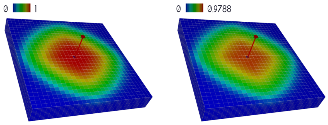
After loading the files using Stratus, we open the field YMFS. As we advance in time, we can observe how the solvent area expands and retreats with a period of six months. The figure below shows the YMFS at the end on the last injection (left) and at the end of the last production (right).

Now load the SGAS field and then click on the J-Icon on the panel top tool bar, and select layer 15, this will generate a slice of the domain through the well:

The figure above shows the SGAS at the end on the last injection (left) and at the end of the last production (right). Even though the well is not in contact with the water, the injected gas displaces the water cyclically below the well.
In this tutorial we are also modelling the temperature variation on the model as a consequence of the injected gas. Now we plot TEMP and again we click on the J-Icon on the panel top tool bar, and select layer 15. Below figures shows that at the end of the last injection period (left) the lowest temperature is lower than the one at the end of the last production period (right). This occurs as the Hydrogen injected is colder than the reservoir, and it gets warmer during the injection/production cycle.

The Hydrogen being injected undergoes a compression (from 70 to 100 Bar) from the point where the temperature is specified (70 Bar, T = 25 C) to the well bottom hole. This results in a small temperature decrease (from 25 C to around 23.5 C), as for these ranges of temperatures and pressures a negative Joule-Thomson (JT) effect is observed. It must be observed that the PFLOTRAN-OGS well model does not account for heat exchanges between the well tubing and its surrounding. To observe this effect we now plot WTEMP (below figure (left)).

During injection the Hydrogen cools down the region around the injector, and it gets warmer as it moves away form the borehole. When switching to production, the Hydrogen extracted gets warmer as time progresses, due to further away warmer gas reaching the well. Hydrogen decompression during production also contributes to the warming up, however this is a secondary effect of less than 1 C, due to a small drawdown pressure of about 10 Bar and a small JT coefficient. Finally, the temperature analysis of a grid block completed by the well, (plot TEMP at cell 15 15 1 above figure right), shows how the region around the well tends to cool down in average with the storage cycles, stabilising to a mean value of about 40 C.
For Hydrogen storage a very important parameter is the storage efficiency, i.e. how much Hydrogen can be recovered from the total injected. To analyse the storage efficiency we want to observe how much Hydrogen is retrieved from that injected. To this end we now plot (below left) WZMFG and WZMFS (total mole fraction of gas and solvent in the well, respectively), and (below right) FNIT and FNPT (total solvent injected and produced).
Below figure (left) shows that in the production phase there is always a certain amount of cushion gas being extracted from the reservoir (red), dropping the storage efficiency. Nonetheless, as the number of cycles progresses the amount of extracted gas is reduced and tends to stabilise over time. This is because, the cushion gas is being effectively replaced by Hydrogen lost in previous cycles. Below figure (right) shows the total amount of Hydrogen produced (green) and injected (red), the gap between both lines at the end of a cycle show the accumulated Hydrogen loss.

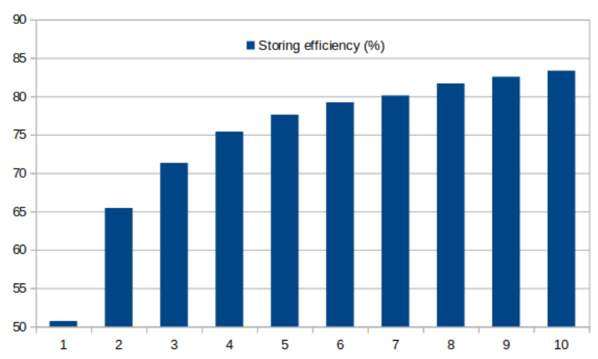
To better study the storage efficiency, the ratio between Hydrogen injected and produced is plotted in the figure below (The numerical values have been obtained using the mas file H2_STORE-mas.dat). The plot shows that the extraction efficiency improves over time, which is expected as the system is generating an area of Hydrogen by displacing the cushion gas. The plot shows that the efficiency of the system rapidly increases from around 50% the first year to above 70% the third year and over 80% efficiency after 10 years.

It is important to note that the storage efficiency of the modeled system depends on the spatial and time resolution used, i.e. artificial diffusion introduced. For Hydrogen storage, the system reverses the direction of the flow, contrary to, for example, CO2 sequestration. Here, diffusion acts by increasing mixing with the cushion gas, i.e. the injected Hydrogen moves further away than what the advectives forces controlled by the well would do without diffusion. This means that when the well changes to be a producer, the Hydrogen has mixed with the cushion gas and therefore the storage efficiency has dropped as the production now includes a mixture of cushion gas and Hydrogen. Thus, artificial diffusion introduced by the mesh resolution and the time-step size further increase the mixing effect, and therefore, decrease the storage efficiency of the model.
To show the impact of artificial diffusion in the storage efficiency, the same model is run by doubling its resolution in space and imposing a maximum time-step size of 20 days (instead of 30 days). To do this, modify the input file h2_store.grdecl to increase the resolution by modifying dimens and dx, dy, dz:
dimens
60 60 20 /

equals
dx    25.0 /
dy    25.0 /
dz    2.5 /
poro  0.2 /
permx 100.0 /
/
Likewise, we need to reposition the wells in H2_STORE.in so we modify the CIJK_D from:
CIJK_D 15 15 1 4
to:
CIJK_D 30 30 1 8
and the maximum timestep size:
MAXIMUM_TIMESTEP_SIZE 20 d at 0. d
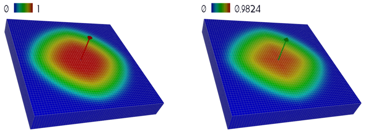
Below figure shows YMFS at the same time as the coarse case. It can be seen, that the Hydrogen region is not only sharper but also smaller than in the coarse case.
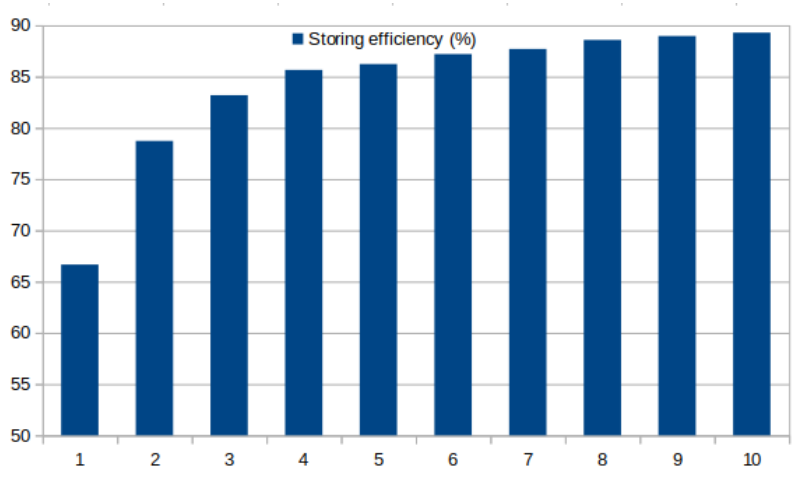
We plot again the the ratio between Hydrogen injected and produced (below figure). It shows that the efficiency of the system is better than in the coarse case. For example, in the first cycle the efficiency is around 65% while in the coarse case it is just above 50%. Equivalently, after 10 years the efficiency in the finer model is almost 90% while in the coarse case it is below 85%.

