Local Grid Refinement (LGR)
Local Grid Refinement (LGR) is a functionality that allows the user to refine the grid in the specified section. Cirrus can do LGR using the keyword CARFIN (local grid refinement). The CARFIN section allows the user to set a grid refinement and also to specify properties within it. Here, we are going to use the static model used in Tutorial 3 – CO2 Storage sites connected to a nearby hydrocarbon field to show how to use LGR. Outline of this section:
Considerations when using LGR
Some key points to take into account when using LGR with Cirrus:
The properties defined in the global grid are imposed to the LGR. For example, the permeability or faults defined in the global grid will be automatically imposed in the LGR. However, there are some fields that need to be defined in the LGR, such as: FIPNUM, Wells and SUMMARY_D data.
Faults cannot be imposed within an LGR. They must be defined in the original grid.
Nested LGR is not available.
An LGR must be isolated from other LGRs, i.e. two different LGRs cannot be defined in adjacent parent cells.
Aquifers cannot be connected to an LGR. The recommended action is to leave the grid blocks attached to an aquifer unmodified.
Setting up a refinement
We are going to start by creating a homogeneous refinement of the original gridblocks.
We add the following in the .grdecl file:
carfin
  rfin 12 16 16 20 1 12 10 10 24 /
endfin
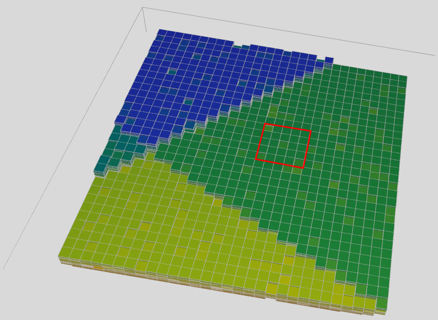
Here, we have named the refinement rfin and we have specified the box of cells:
i-dir: 12 to 16
j-dir: 16 to 20
z-dir: 1 to 12
In this example we set up exactly twice the number of elements: 10, 10 and 24 instead of 5, 5, 12. We now obtain the following grid:
If we wanted a finer refinement, we only need to change the new number of elements in the LGR. To show this, we are going to do another refinement. We therefore change the number of elements:
carfin
  rfin 12 16 16 20 1 12 20 20 24 /
endfin
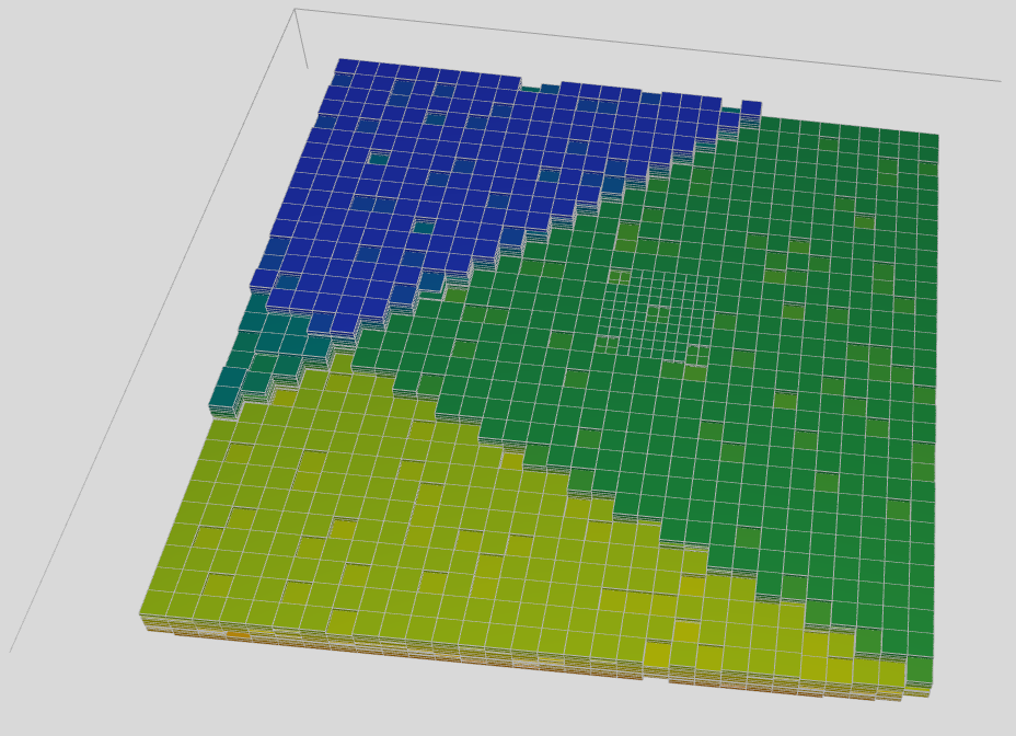
Here, we have further refined in i- and j- dir but we have left intentionally the z-dir to be the same as in the previous refinement. We now obtain the following grid:
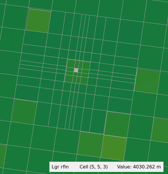
In the previous examples we have set an isotropic refinement, i.e. the new element size was obtained by splitting equally the original grid. Nonetheless, that is not necessary and the refinement can be anisotropic, i.e. different in space. We are going to set an example where the grid is finer at the horizontal centre of the refinement and coarsens the further away it is from the centre. Thus, we need to use the keywords HXFIN/HYFIN and NXFIN/NYFIN (If we wanted to do the vertical as well, we would need as well HZFIN/NZFIN):
carfin
  rfin 12 16 16 20 1 12 10 10 24 /
  nxfin
    1 2 4 2 1 /
  nyfin
    1 2 4 2 1 /
  hxfin
    10 8 5 2 1 1 2 5 8 10 /
  hyfin
    10 8 5 2 1 1 2 5 8 10 /
endfin
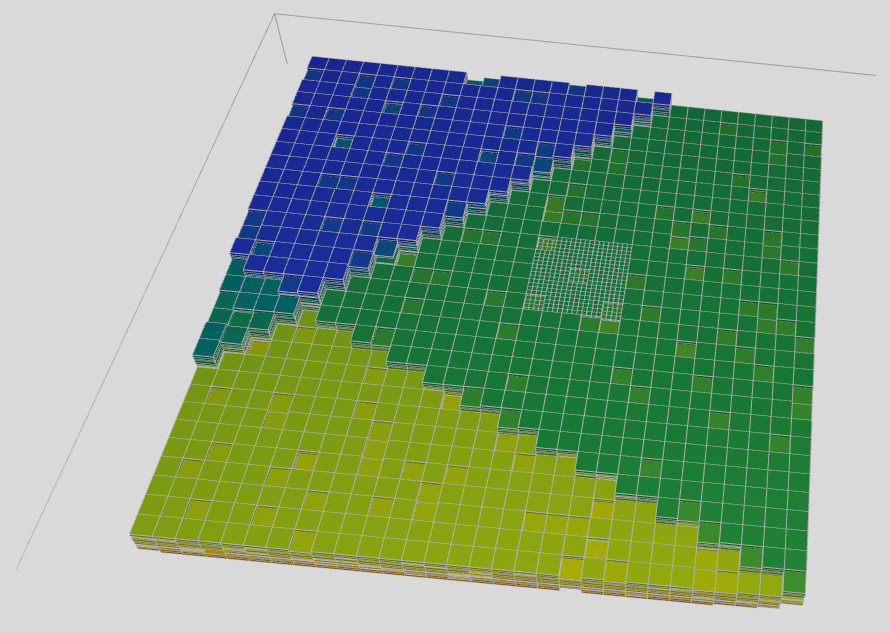
with the above we obtain the following:
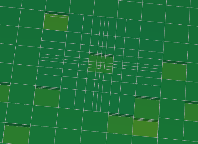
It can be seen that we have obtained the grid we were looking for, with a gradient of grid-block size going from the center of the LGR. If we now analyse the commands, we can note the following:
NXFIN/NYFIN: These keywords work on the original coarse grid. We have specified that the outer original grid-blocks are not refined (1), the contiguous to be split into two (2) and the inner one to be split into four (4)
HXFIN/HYFIN: These keywords work on the refined grid and expect values defining the relative size of the refinement. The different numbers therefore provide the relative size between the different refined elements.
Placing a well in an LGR
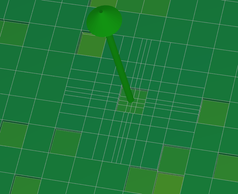
Following the previous example, we are going to place a well within the LGR rfin in the position highlighted:
To do this we need to use the keyword CIJKL_D instead of CIJK_D. Thus, we modify the CCS_3DF.in file adding a new well as follows:
WELL_DATA LGR_prod
  CIJKL_D 5 5 3 3 rfin
  DIAMETER 0.1524 m
  WELL_TYPE PRODUCER
  BHPL      150 Bar
  TARG_WSV  1000 m^3/day
  DATE 1 JAN 2033
  SHUT
END
In this case, the coordinates need to be introduced using the LGR coordinates and also specify the LGR name (as there can be, potentially, many). We obtain the well in the desired position:
It is important to note that CIJKL_D can also provide values per completion as it is done for CIJK_D:
CIJKL_D 5 5 3 3 rfin Z CCFUSER 3.0 METRIC
Setting properties within an LGR
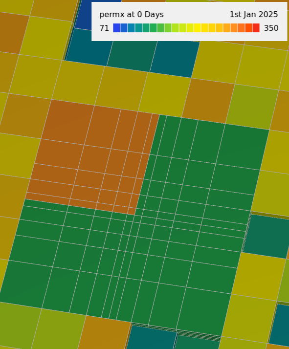
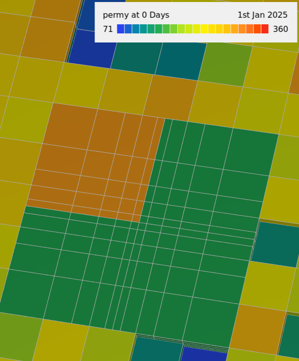
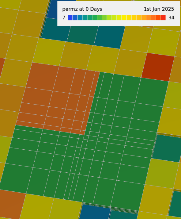
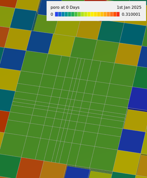
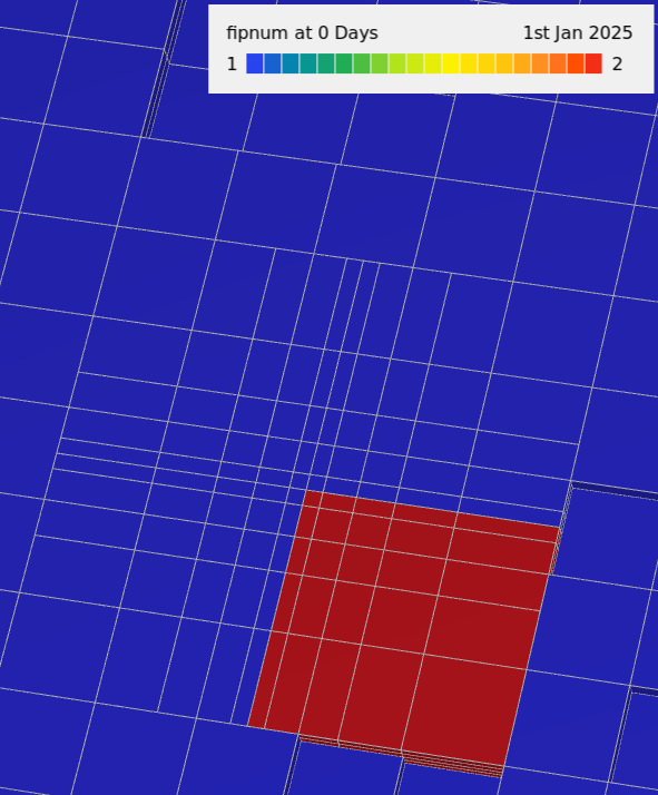
Petrophysical properties such as permeability, porosity or fields such as ACTNUM or FIPNUM can be modified within an LGR. The user can do this as it would normally do using the keywords described in GRDECL grids within the CARFIN/ENDFIN section (It is important to note that we must work in the LGR coordinates). In the next example we define FIPNUM, porosity and permeability within the LGR using different keywords:
carfin
  rfin 12 16 16 20 1 12 10 10 24 /
  nxfin
    1 2 4 2 1 /
  nyfin
    1 2 4 2 1 /
  hxfin
    10 8 5 2 1 1 2 5 8 10 /
  hyfin
    10 8 5 2 1 1 2 5 8 10 /

  equals
    permx 150 1 10 1 10 1 24 /
    fipnum 1 1 5  1 5  1 24 /
    fipnum 2 6 10 6 10 1 24 /
  /
  add
    permx 150 1 5 1 5 1 24 /
  /
  copy
    permx permy /
    permx permz /
  /
  multiply
    permz 0.1 /
  /
  poro
    2400*0.11 /
endfin
Obtaining the following:
Block report within an LGR (SUMMARY_D/SUMMARY_Z)
Normally, to extract the data within a gridblock the user can use SUMMARY_D/SUMMARY_Z to select which gridblock and which property is going to be exported to the summary file. However, when using LGR one must use the LGR coordinates and place the name of the LGR after the coodinates. The following shows an example requesting different values within the LGR rfin at cell (5,5,3):
OUTPUT
  MASS_BALANCE_FILE
   PERIODIC TIMESTEP 1
  END
  ECLIPSE_FILE
    PERIOD_SUM TIMESTEP 5
    PERIOD_RST TIMESTEP 20
    WRITE_DENSITY
    WRITE_RELPERM
    DATES 1 JAN 2027 ! CO2 injection starts
    DATES 1 JAN 2031 ! CO2 injection stops
    DATES 1 JAN 2033 ! Production stops
    DATES 1 JAN 2225 ! Simulation ends
    OUTFILE
    SUMMARY_D
      BPR   5 5 3 rfin
      BGSAT 5 5 3 rfin
      BWSAT 5 5 3 rfin
      BDENG 5 5 3 rfin
      BDENW 5 5 3 rfin
      BVGAS 5 5 3 rfin
      BVWAT 5 5 3 rfin
    END_SUMMARY_D
  END
  LINEREPT
END
Note that the convention for the outputted field names is the same as for the normal case (SUMMARY_D/SUMMARY_Z) but an L before and followed by _*LGRNAME*. For example in this case we would obtain LBDGAS_RFIN instead of BDGAS.