Tutorial 1 - CO2 Storage in Saline Aquifers – Long term effects
You will learn about:
setting up the module to run a CO2 storage problem on a simple grid
setting up water and CO2 characterisation using the software internal correlations
visualising CO2 concentration in brine
analysing output files to quantify the CO2 solution and residual trapping mechanisms
To run this tutorial you will need the following:
Three input files are used for this tutorial, these can be downloaded at the following links:
These are available as a zip file:
In addition you will need:
Stratus or ResInsight installed in your local machine
Tutorial sections:
Problem description
The CO2 storage problem you are going to model is a cross section, which extends 5000 m in the horizontal direction and 400 m in the vertical direction, with the top located at a depth of 800 m. Hydrostatic pressure and a geothermal gradient of 3 C/100m describes the unperturbed conditions of the reservoir before injection starts.
The reservoir is initially saturated in brine and 1Mt/year of CO2 is injected at 1000 meters depth, right in the middle of the domain, for 6.85 years. The simulation is then let run for 5000 years. A producer operating at constant pressure is completed in the bottom layer to emulate a deep aquifer underneath and avoid pressure build up.
Although this is a two-dimensional model, it is run as three-dimensional, with a single grid block in the span-wise direction, giving the cross section a thickness of 1000 m.
Setup of the input file
Download CCS_LT.in, ccs_lt.grdecl and co2_dbase.dat and put them in the folder where you are going to run the tutorial. Note that the input deck name is in capitals, so the simulator output files will all also be in capital letters including their extension, e.g. CCS_LT.UNRST. This avoids issues when loading output files with ResInsight (capital cases are not required for Stratus).
Open the input CCS_LT.in with a text editor. Instructions are organised by blocks, each starting by a keyword and terminated by “END” or the forward slash “/”. Line starting by “!” or “#” are comments and ignored by the simulator.
Simulation
In the SIMULATION instruction block, you must select the mathematical model to simulate a CO2 storage problem in saline aquifer, i.e. the GAS_WATER mode mode. This models CO2 solubility in brine and a vapour phase that can have both CO2 and water steam. The problem of this tutorial is treated as isothermal, therefore the ISOTHERMAL flag must be included to overwrite the default thermal setting.
SIMULATION
  SIMULATION_TYPE SUBSURFACE
  PROCESS_MODELS
    SUBSURFACE_FLOW Flow
      MODE GAS_WATER
      OPTIONS
        ISOTHERMAL
        RESERVOIR_DEFAULTS
      /
    / ! end of subsurface_flow
  / ! end of process models
END  !! end simulation block
Be sure RESERVOIR_DEFAULTS is always included, as this specifies tuned values for all numerical parameters required by the simulator.
Grid
The simulation grid and its static properties (permeabilities, porosities, etc.) are defined via an include file inserted in the following block:
GRID
  TYPE grdecl ccs.grdecl
END
To see the grid definition open with a text editor the ccs.grdecl file, which follows the ECLIPSE format and syntax:
dimens
50 1 100 /

equals
tops 800 4* 1 1 /
/

equals
dx    100   /
dy    1000  /
dz    4     /
poro  0.3   /
permx 500.0 /
/

copy
permx permy /
permx permz /
/

multiply
permz 0.1 /
/

dpcf
0.8 1 /
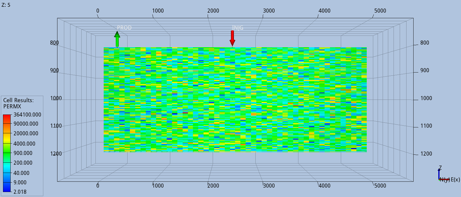
The instructions above define a grid of 5000 blocks: 50 in the horizontal direction (X), 100 in the vertical direction (Z), and 1 block for the cross section thickness (Y). DX= 100m and DZ = 4 define the discretization and DY=1000 m is the cross section thickness. The top layer is located at a depth of 800m. A base permeability of 500 mD is specified, and the vertical permeability is obtained applying a 0.1 multiplier. A random permeability heterogeneity is introduced using dpcf, while the porosity is given a 0.3 constant value.
Time
In the TIME block you must specify the final time of the simulation. This can be given as the time to simulate starting from zero:
TIME
  FINAL_TIME 5000 y
  INITIAL_TIMESTEP_SIZE 0.1 d
  MAXIMUM_TIMESTEP_SIZE 50 d at 0 d
  MAXIMUM_TIMESTEP_SIZE 250 d at 1 y
  MAXIMUM_TIMESTEP_SIZE 1000 d at 25 y
  MAXIMUM_TIMESTEP_SIZE 10000 d at 250 y
END
The study will start from time zero and simulate 5000 years into the future. As most reservoir simulator post-processors use dates to display results, a default start date is linked to time zero and written in the output files, this is “1 JAN 2000”. PFLOTRAN-OGS also accepts start and final dates, these will be introduced in Tutorial 3.
In the TIME instruction block you can optionally specify time step constrains. In this example the following are set:
the initial time step is set to 0.1 days
the time step is limited to 50 days at time zero when the simulation starts
the maximum time step is increased to: 250 days when the simulation reaches 1 year, 1.000 days when the simulation reaches 25 years, and 10.000 days when the simulation reaches 250 years. It is highly recommended to set up maximum time step values based on the physics being modelled, as this can improve the simulation performance significantly.
Output
In OUTPUT you can define the ECLIPSE_FILE block that instructs the simulator to write Eclipse restart and summary files, suitable for post-processing packages that can read this format:
OUTPUT
  MASS_BALANCE_FILE
   PERIODIC TIMESTEP 1
  END
  ECLIPSE_FILE
    TIMES d 2500 1825000
    PERIOD_SUM TIMESTEP 5
    PERIOD_RST TIMESTEP 25
    OUTFILE
  END
  LINEREPT
END
In this example, reporting times are specified for the restart and the summary files (i.e. every 5 and 25 time steps respectively). Two additional reporting times are requested: 2500 days, when the injection stops, and 1825000 (5000 years) when the simulation ends. OUTFILE asks the simulator to print to the CCS_LT.out file the fluid-in-place report and gas phase partitioning to quantify solution and residual trapping.
Field gas mass in place (fgmip), field gas mass in gas phase (fgmgp), field gas mass dissolved in the aqueous phase (fgmds), field gas mass trapped in the gas phase (fgmtr), and field gas mass in the mobile gas phase (fgmmo) are always output to the summary file when using the GAS_WATER mode.
Material Property
In this block you must specify material properties constant over the entire domain.
MATERIAL_PROPERTY formation
  ID 1
  ROCK_COMPRESSIBILITY    4.35d-5 1/Bar
  ROCK_REFERENCE_PRESSURE 1.0     Bar
  CHARACTERISTIC_CURVES ch1
/
The rock compressibility is given a typical value of \(4.35 \times 10^{-5}\) 1/Bar.
A set of characteristic curves (saturation functions) called “ch1”, which will be defined later, is associated to this material.
ID must be given 1 as there is only one material. This entry is compulsory. The material property name, “formation” in this example, is also required.
Characteristic curves (Saturation function)
In the characteristic curve block, you must define a valid set of saturation functions. For the gas water model the set can be formed by two tables, SWFN and SGFN.
SWFN has water saturation in the first column, water relative permeability in the second and water-gas capillary pressure in the third.
SGFN has gas saturation in the first column, gas relative permeability in the second, while the third column, which expects capillary pressure between gas and oil, is not used.
The name of the set of curves, “ch1”, must be the same specified in MATERIAL_PROPERTY.
CHARACTERISTIC_CURVES ch1

 TABLE swfn_table
   PRESSURE_UNITS Bar
   SWFN
     0.0    0    0.4
     0.1    0    0.3
     0.9    1    0.2
     1.0    1    0.1
   /
 END

 TABLE sgfn_table
  PRESSURE_UNITS Bar
    SGFN
     0.0     0      0
     0.10    0.0    0
     0.255   0.15   0
     0.51    0.4    0
     0.765   0.8    0
     1.0     1.0    0
    /
 END

/
Fluid Properties
For the fluid properties, select the model that describes the gas component as real CO2, and define the surface densities for water and gas. Diffusion coefficients and brine halite concentration will be defaulted if not entered.
FLUID_PROPERTY
  PHASE LIQUID
  DIFFUSION_COEFFICIENT 2.0d-9
/
FLUID_PROPERTY
  PHASE GAS
  DIFFUSION_COEFFICIENT 2.0d-5
/

BRINE 1.092 MOLAL

EOS WATER
 SURFACE_DENSITY 1000.0 kg/m^3
END

EOS GAS
  SURFACE_DENSITY 1.0 kg/m^3
  CO2_DATABASE co2_dbase.dat
END
With the instructions above the brine properties are computed using water tables with a correction for salinity and dissolved CO2. CO2 properties are computed using a database defined by an include file, co2_dbase, provided with this tutorial.
The phase composition are computed with internal correlations of the GAS_WATER model.
Equilibration
Instruct the simulator on how to initialise the study. This can be done by defining an hydrostatic equilibration using the EQUILIBRATION data block:
EQUILIBRATION

  PRESSURE 80.0 Bar
  DATUM_D  800 m

  GAS_IN_LIQUID_MOLE_FRACTION 0.0

  TEMPERATURE_TABLE
    D_UNITS m
    TEMPERATURE_UNITS C !cannot be otherwise
    RTEMPVD
     800  29
     1000 35
     1200 41
    /
  END

/
The hydrostatic pressure equilibration requested above sets a pressure of 80 Bars at a depth of 800m, and an initial CO2 concentration in brine given in terms of molar fraction equal to 0. The initial temperature profile over depth is specified by means of temperature table assigning different temperature at different depths (e.g. 29 C at 800 m, etc.)
Although the simulator is running in isothermal mode, the temperature variation with depth is taken into account to compute all fluid flow properties.
Wells
You can use WELL_DATA to define a well, its location and its operating schedule. In this example you must include an injector and a producer:
WELL_DATA injg
  WELL_TYPE GAS_INJECTOR
  BHPL     1000    Bar
  TARG_GM 1.0 Mt/y
  CIJK_D   25 1 50 50
  TIME 2500 day
  SHUT
END

WELL_DATA prod
  WELL_TYPE PRODUCER
  BHPL     120.5    Bar
  TARG_WSV 10000 m^3/day
  CIJK_D   1 1 100 100
  […………………]
  CIJK_D  50 1 100 100
END
In the instructions above, the well locations are defined specifying the completed blocks using the IJK logical coordinates, and the operational schedule specifying target types and event TIMEs.
The gas injector is located in the middle of the cross section (block 25,1,50), with an injection target of 1 Megatonne of CO2 per year (Mt/y). After injecting 2500 days (~6.85 years), the injector is shut.
The producer operating with a bottom hole pressure of 120.5 bars is completed in the bottom layer to emulate a deep aquifer underneath and avoid pressure build up.
Run the simulation
Run the simulation set up for this tutorial on your preferred environment. Open one of the links below on a new tab, so you can continue following the instructions to analyse the result in this page.
Analyse the results
The simulator outputs the ECLIPSE restart and summary files (CCS_LT.RST, CCS_LT.UNSMRY, CCS_LT.SMSPEC), which you can load with any post-processor supporting this format.
Continue this tutorial analysing the results using Stratus or ResInsight, clicking one of the links below:
Analyse the CCS_LT results with Stratus
Eclipse restart files
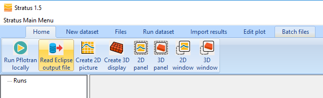
Launch Stratus. In the top-left corner click the Read Eclipse Output File icon:
Browse the folder where you run the case, then select and open the .GRID file
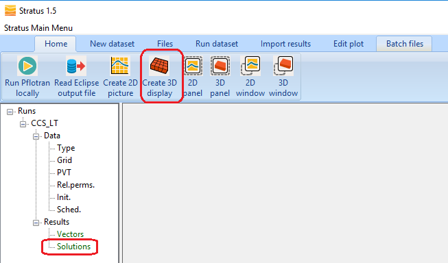
Click the Create 3D Display icon or select Solution under the CCS_LT case:
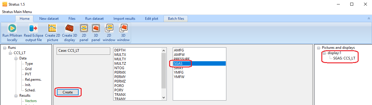
Then select SGAS, click Create, and select the SGAS display on the right-side tree menu:
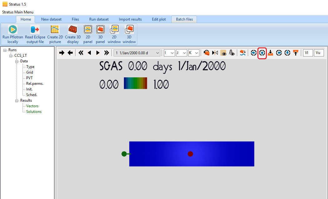
Then click on the Y-positive Icon on the Panel top tool bar (highlighted by a red circle above), and advance the time to Nov 2006 (end of the injection):
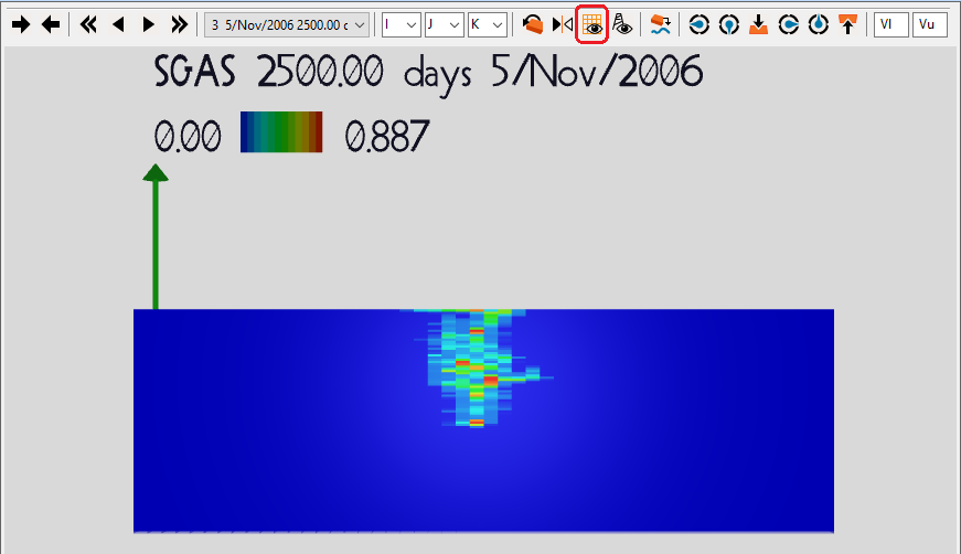
To move the domain hold down the right button of the mouse as you move it, to zoom in and out hold the middle button of the mouse as you move it. In the top menu click on the grid view icon (highlighted by a red circle above) to toggle on/off the grid.
At the end of the injection, the gas is distributed in the region around and above the injector as CO2 migrates towards the top layer.
Advance the time to the end of the simulation, ~5000 years (Sep 6996).
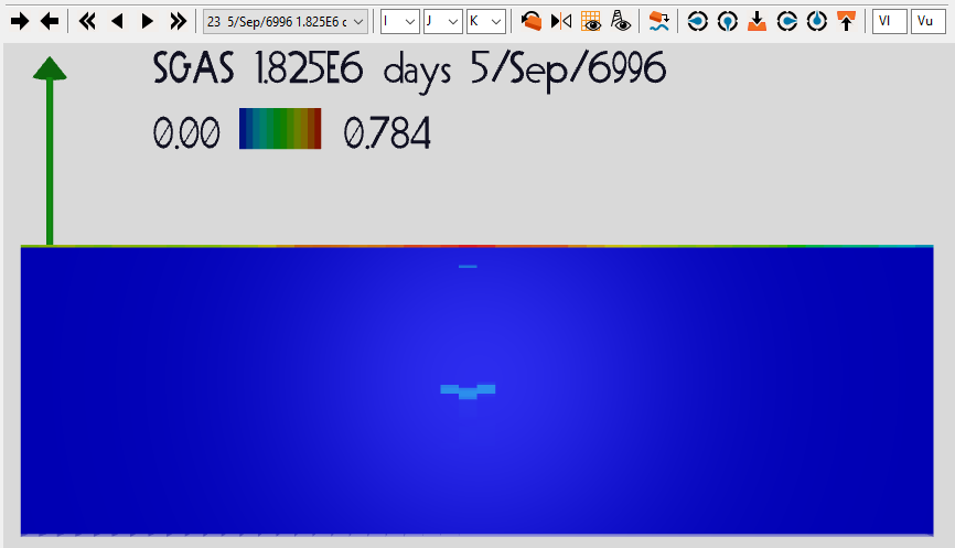
After 5000 years a thin layer of gas is still present in the top layer, while most of the CO2 has dissolved in brine. You can better visualise the dissolved CO2 by creating a 3D Display of AMFG (aqueous mole fraction of gas). To do so repeat the same steps followed to create the SGAS 3D display, but select AMFG instead:
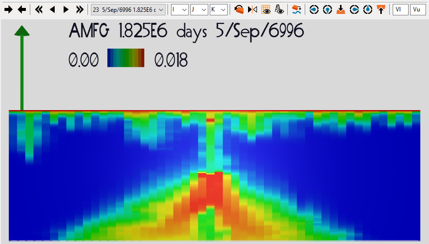
This plots the concentration of CO2 in brine, showing how the density-driven fingers are sinking the CO2 towards the bottom of the aquifer.
Line Graphs of dissolved, trapped and mobile gas
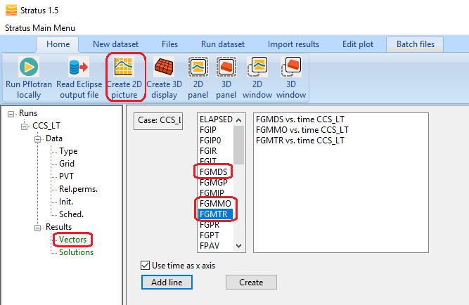
In order to visualise how the different trapping mechanisms evolve over time, you will now create plots vs time of: field gas mass dissolved in the aqueous phase (fgmds), field gas mass trapped in the gas phase (fgmtr), field gas mass in the mobile gas phase (fgmmo). To do this click on the Create 2D Picture Icon, or select Vectors under the CCS_LT case. Then select one at time the following three variables: FGMDS, FGMMO and FGMTR. For each selection click Add Line to compose a plot with three curves:
Once all three lines appear in the central box, click Create. This will add to the right-side tree menu a Picture (graph). To display this graph, click on picture1 on the right-side tree menu or on the 2D Panel icon. Finally, if you want to switch the x-axis format from days to dates, use the clock/calendar icon in the toolbar located at the top of the 2D panel:
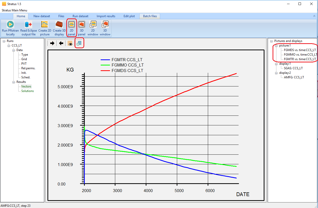
The plots above shows how the amount of gas dissolved in brine increase over time (red line), while the trapped (blue line) and the mobile gas (green line) reduce.
You can check the numeric values of the mass balance and CO2 budgets at a given time in the output file.
Analyse the CCS_LT results with ResInsight
Eclipse restart files
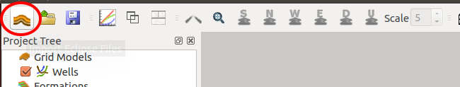
Launch ResInsight. In the top-left corner click the open case icon:
Browse the folder where you run the case, then select and open the .GRID file, you should see the following:
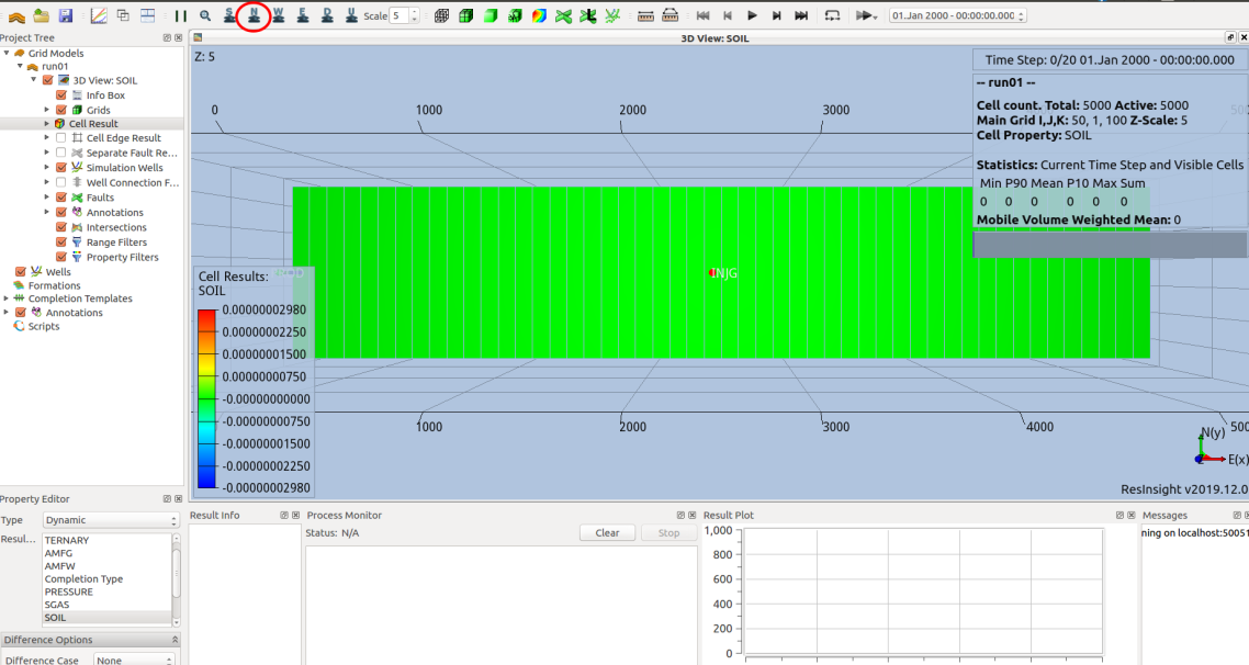
On the top menu, select the North View, indicated by a capital N (red circle in the picture above). On the left-side menu uncheck the Info Box to clear the information box in the panel and select Cell Result. In the bottom-left menu, within Property Editor, select SGAS. In the top menu click on the blue cuboid icon to visualise the contour without the grid, and advance the time until November 2006:
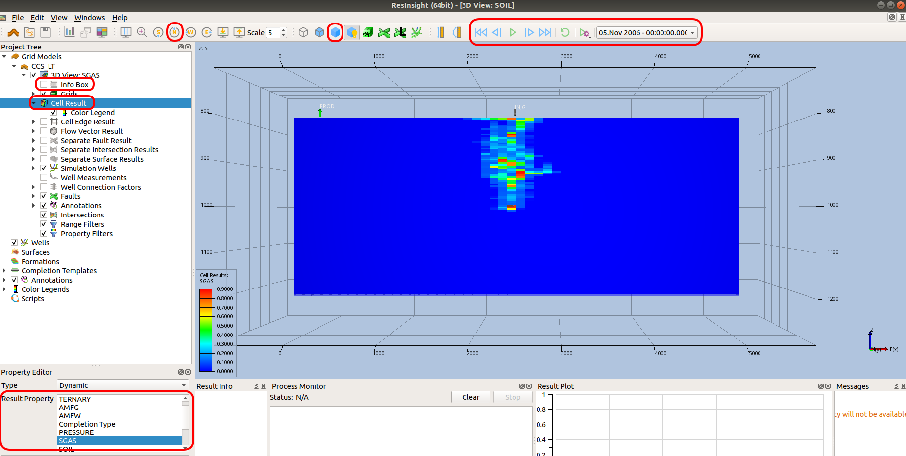
To move the domain hold down the right button of the mouse as you move it, to zoom in and out hold the left button of the mouse as you move it.
The SGAS contour above above shows the gas saturation at the end of the injection.
Then advance the time to the end of the simulation, ~5000 years (Sep 6996).
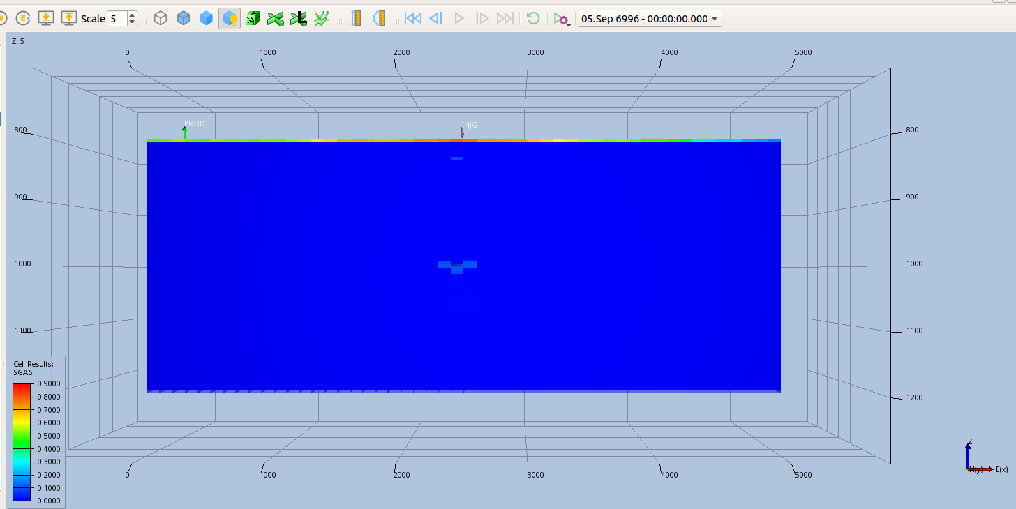
After 5000 years a thin layer of gas is still present in the top layer, while most of the CO2 has dissolved in brine. You can better visualise the dissolved CO2 by selecting AMFG (aqueous mole fraction of gas) in the Property Editor:
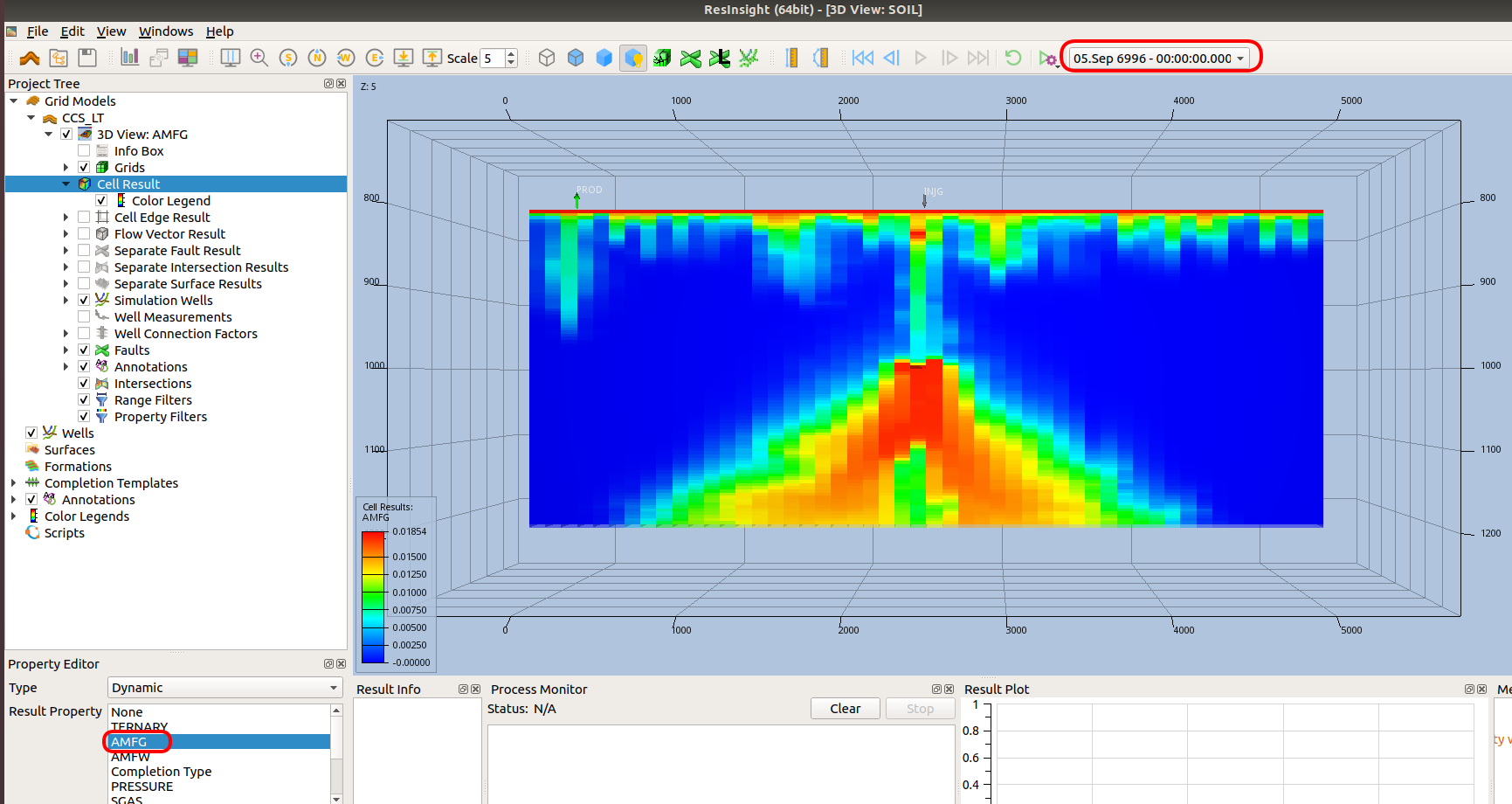
This plots the concentration of CO2 in brine, showing how the density-driven fingers are sinking the CO2 towards the bottom of the aquifer.
Line Graphs of dissolved, trapped and mobile gas
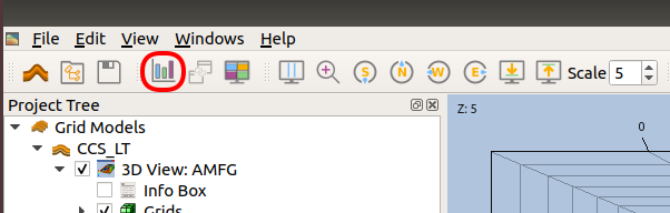
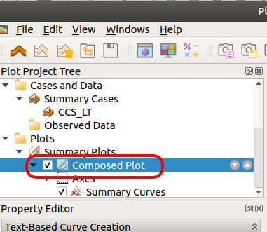
In order to visualise how the different trapping mechanisms evolve over time, you will now create plots vs time of: field gas mass dissolved in the aqueous phase (fgmds), field gas mass trapped in the gas phase (fgmtr), field gas mass in the mobile gas phase (fgmmo). To do this open the ResInsight plot editor, clicking on the graph icon (see red circle below):
Then right click on Composed Plot, and select Edit Summary Plot.
In the editing window that opens do the following selections:
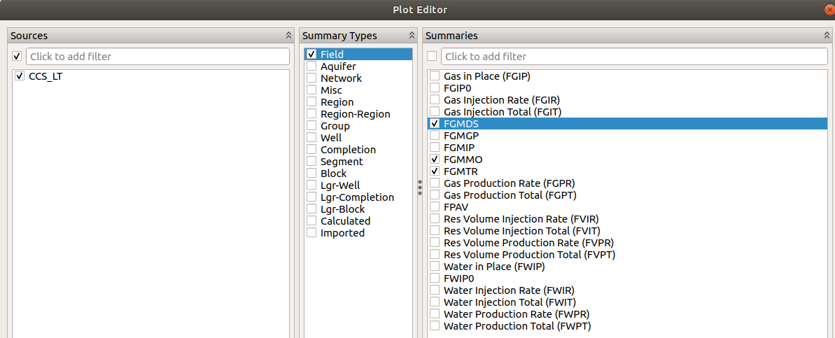
Then click ok:
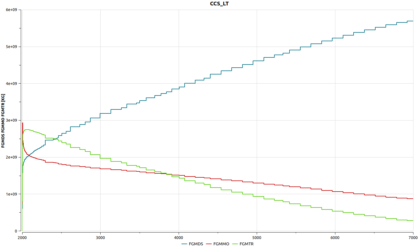
The plots above shows how the amount of gas dissolved in brine increase over time (blue line), while the trapped (green line) and the mobile gas (red line) reduce.
You can check the numeric values of the mass balance and CO2 budgets at a given time in the output file.
Output file
Open the file CCS_LT.out with a text editor, and search for “2500.000 days”, i.e. end of the injection. You will see the fluid-in-place (FLIP) report and the gas phase partitioning:
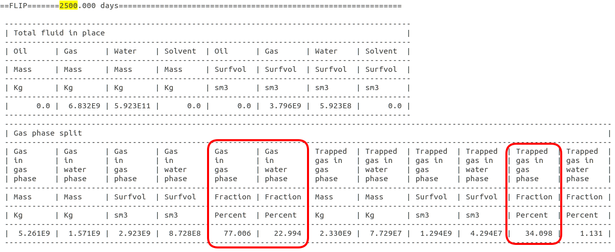
At the end of the injection about 23% of the total CO2 is dissolved in brine, and 77% is in the gas phase. About 34% of the CO2 is trapped as immobile gas.
If you now scroll down to the end of the output file, you can see the same report at the end of the simulation (5000 years, i.e. 1.825 \(\times 10^6\) days):
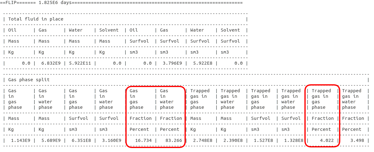
83.3% of the CO2 has dissolved in brine (solution trapping) and 16.7% is still in the gas phase. About 4% of the CO2 is trapped as immobile gas.