Tutorial 2 - CO2 Storage in saline aquifers – Non-isothermal effects
You will learn about:
setting up a CO2 storage problem that models temperature effects
setting up analytical aquifers
setting up and display grid block reports
analysing results of thermal CO2 storage studies
using restart files
To run this tutorial you will need the following:
Five input files are used for this tutorial, these can be downloaded at the following links:
These are available as a zip file:
In addition you will need:
Stratus or ResInsight installed in your local machine
Tutorial sections:
Problem description
The problem models a cold injection of CO2 into a target layer with a horizontal extension of 2x2 km and a thickness of 50 m. Assuming the problem is symmetric in x and y, you can model only one quarter of the domain.
The reservoir is initially saturated with brine in hydrostatic equilibrium, and the vertical temperature distribution follows a geothermal gradient of 3 C/100 m. The caprock and under-burden, located at a depth of 1200 and 1250 meters, are assumed to have zero permeability.
1Mt per year of CO2 is injected for 7 years through a vertical well that completes five layers, from a depth of 1225 to 1250 m. The CO2 enters the reservoir at about 15 C, where it finds an ambient temperature of ~52 C, cooling significantly the region around the injector. The simulation is continued for ~500 years after the injection to assess the time needed by the reservoir to recover its initial temperature. The aquifer surrounding the injection area is described by an analytical model.
Two vertical portions of 50 meter for the caprock and the overburden are included in the model to account for the diffusive heat exchange with the target layer.
Setup of input file
With a text editor open the input deck provided for this tutorial, INJ_TH.in. The explanation below discuss only sections with instructions not covered in Tutorial 1.
Simulation
Select the GAS_WATER mode mode, and be sure the ISOTHERMAL card is removed, as the software runs with the temperature option switched on by default.
SIMULATION
  SIMULATION_TYPE SUBSURFACE
  PROCESS_MODELS
    SUBSURFACE_FLOW Flow
      MODE GAS_WATER
      OPTIONS
      RESERVOIR_DEFAULTS
      /
    / ! end of subsurface_flow
  / ! end of process models
END  !! end simulation block
Grid
In the grid files, set zero permeability to the caprock and under-burden using a 0 multiplier:
dimens
20 20 16 /

[………………]

multiply
permx 0.0 4*  1  3 /
permx 0.0 4* 14 16 /
/
Time
Specify 7 years as the final time of the simulation, using the FINAL_TIME keyword:
TIME
  !uses default start date JAN 2000
  FINAL_TIME 7 y
  INITIAL_TIMESTEP_SIZE 0.1 d
  MAXIMUM_TIMESTEP_SIZE 100 d at 0 d
END
Output
Within the ECLIPSE_FILE block, specify the times at which the restart files are required (1, 2, 3, 4, 5, 6, 7 years).
Add the statements to output the density and viscosity (WRITE_DENSITY, WRITE_VISCOSITY), as it will be interesting to observe how these two parameters change with temperature in the region around the injector. Ask for a report vs time for pressure (BPR), gas saturation (BGSAT), and temperature (BTEMP) in two specific grid blocks (1,1,10) and (7,7,4). The first block is one of those completed by the injector, the second block is an observation just below the caprock, located ~1000 m away from the injector. The grid block reports are included in the set of instructions started by SUMMARY_D and terminated by END_SUMMARY_D.
OUTPUT
  MASS_BALANCE_FILE
   PERIODIC TIMESTEP 1
  END
  ECLIPSE_FILE
    TIMES y 1 2 3 4 5 6 7
    PERIOD_SUM TIMESTEP 1
    OUTFILE
    WRITE_DENSITY
    WRITE_VISCOSITY
    SUMMARY_D
      BPR    1  1  10
      BGSAT  1  1  10
      BVGAS  1  1  10
      BVWAT  1  1  10
      BDENG  1  1  10
      BDENW  1  1  10
      BTEMP  1  1  10
      BGSAT  7  7   4
      BPR    7  7   4
      BTEMP  7  7   4
    END_SUMMARY_D
  END
  LINEREPT
END
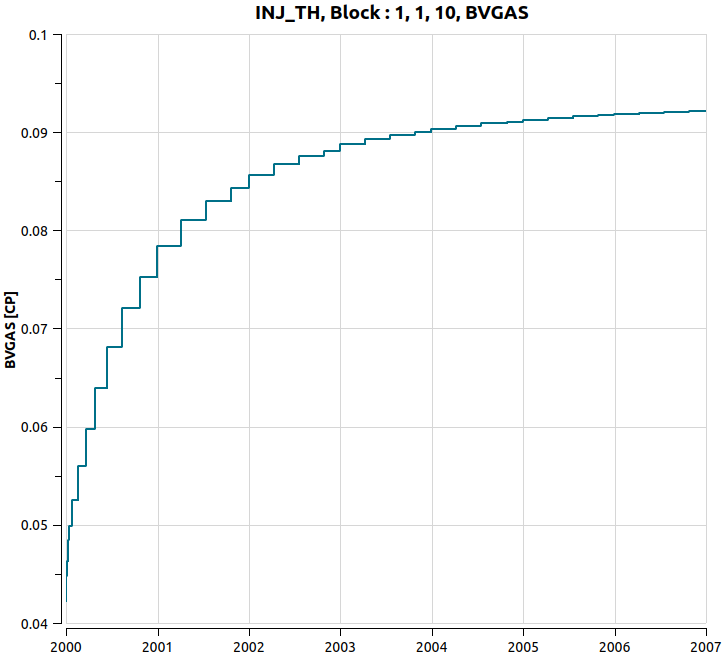
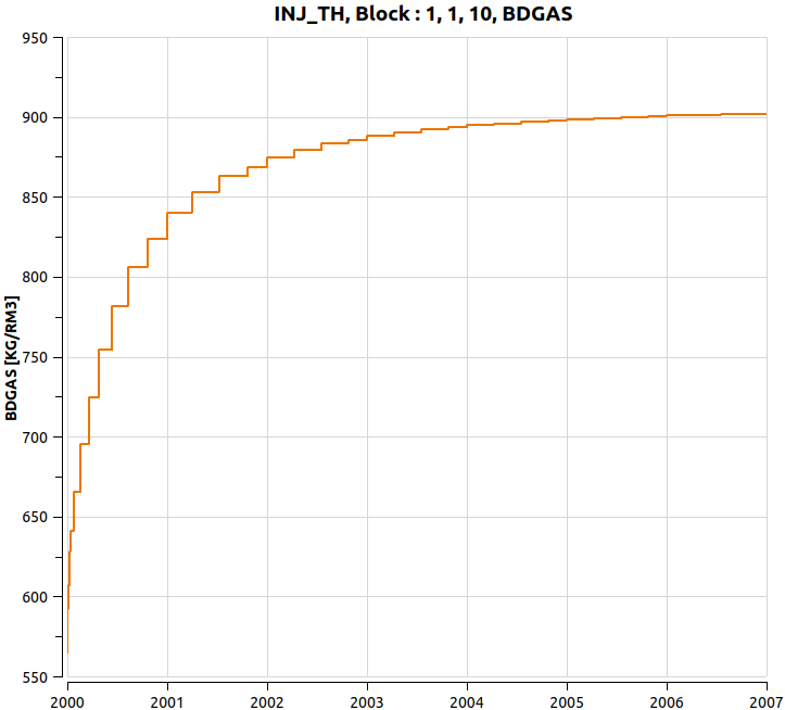
The output definition above also includes reports for gas viscosity (BVGAS), water viscosity (BVWAT) , gas density (BDENG) and water density (BDENW) for the grid block (1,1,10).
Material Property
Enter the rock density (2350 kg/m3), the specific heat capacity (1000 J/(kg-K) ) and the thermal conductivities for CO2 saturated rock (1.6 W/(K-m) ) and for brine saturated rock (4.3 W/(K-m)), these are input needed for a thermal run.
MATERIAL_PROPERTY formation
  ID 1
  ROCK_DENSITY 2.350d3          kg/m^3
  SPECIFIC_HEAT 1.0d3           J/kg-C
  THERMAL_CONDUCTIVITY_DRY 1.6  W/m-C
  THERMAL_CONDUCTIVITY_WET 4.3  W/m-C
  ROCK_COMPRESSIBILITY    4.35d-5 1/Bar
  ROCK_REFERENCE_PRESSURE 1.0     Bar
  CHARACTERISTIC_CURVES ch1
/
Note that the thermal conductivity of each grid block will be computed taking a saturation-weighted average (see the MATERIAL_PROPERTY card), which combines the two thermal conductivities given for the brine-saturated (WET) and brine-unsaturated (DRY) rock.
Thermal boundaries
To ensure the naturally occurring thermal gradient is preserved over time, fix the temperature at the top and bottom of the over- and under-burdens to their initial values. You can do this by including two TBC_DATA blocks that specifies a temperature vs depth distribution equal to the one used to initialise the study.
TBC_DATA tbctop
  TEMPVD m C
     1150 50
     1300 54.5
  END TEMPVD
  CONN_D 1 20 1 20 1 1 Z-     !top faces
END

TBC_DATA tbcbot
  TEMPVD m C
     1150 50
     1300 54.5
  END TEMPVD
  CONN_D 1 20 1 20 16 16 Z+ ! bottom faces
END
The temperature values at the top and bottom boundaries will be interpolated from the table values. This is equivalent to fixing constant temperatures if the top and bottom layers are flat. However, in case of layers that have variable depth, the table approach fixes the temperature boundary values to their initial values.
CONN_D defines the layers and faces to which the thermal boundary is assigned. Inter-grid-block faces are skipped.
Aquifer
Define two Carter-Tracy analytical aquifers using the AQUIFER_DATA instruction block, and apply one to the each side opposite to the injectors (north and east). You can specify the cells and the faces to which the aquifer will be connected using CONN_D.
AQUIFER_DATA north
  BACKFLOW
  DEPTH     1225.0 m
  THICKNESS  50 m
  RADIUS    3000.0 m
  PERM      300  mD
  TEMPERATURE 53.0 C
  COMPRESSIBILITY 2.0E-9 1/Pa
  POROSITY  0.3
  VISCOSITY 1 cP
  CONN_D 1  20 20 20 4 13 Y+
END

AQUIFER_DATA east
  BACKFLOW
  DEPTH     1225.0 m
  THICKNESS  50 m
  RADIUS    3000.0 m
  PERM      300  mD
  TEMPERATURE 53.0 C
  COMPRESSIBILITY 2.0E-9 1/Pa
  POROSITY  0.3
  VISCOSITY 1 cP
  CONN_D 20 20  1 20 4 13 X+
END
The instructions above define two aquifers located at a depth of 1225 m, 50 m thick, with an internal radius of 3000 m. The other parameters specified for the aquifers are: porosity (0.3), permeability (300 mD), viscosity (1 cP) and temperature (53 C).
The connections to the boundaries are specified in two separate instruction lines, one for each side. The keyword BACKFLOW indicates that fluid can flow from the reservoir to the aquifer, as by default only flow from the aquifer to the reservoir is allowed.
Temperature and CO2 concentration for the aquifer are required in case of fluid flow from the aquifer to the reservoir. You must enter the aquifer temperature (53 C), while you can default the CO2 concentration (to zero if not found).
Wells
You want to define a vertical gas injector located in centre of the reservoir with completions in the 5 deepest layers, and injecting one million metric tonne of CO2 per year (Mt/y). As symmetry is assumed for this case, and only one quarter of this reservoir is modelled, use WELL_DATA to define a vertical gas injector in one corner (I=1,J=1,K=9,13), and set the injection rate to 0.25 Mt/y. To reflects that the well injects only in a radial range of 90° over 360°, impose a THETA_FRACTION of 0.25, which will reduce the completion connection factors accordingly.
You must specify the pressure and temperature of the CO2 being injected, in a point where these parameters are known, as PFLOTRAN-OGS needs them to compute the energy (enthalpy) entering the reservoir. From the point where pressure and temperature are specified to the bottom hole conditions of the injector, the simulator assumes an isenthalpic process, neglecting heat exchanges of the well tubing with the surroundings rock, as well as changes in potential and kinetic energies.
With the present model, to get a realistic approximation of the energy entering the reservoir, you will need to know the bottom hole temperature (BHT) and pressure (BHP). In general, the operational BHP and BHT vary, but for prolonged and continuos injections, they tend to stabilise after the initial startup. You can get a reasonable estimate of the stable BHP with a preliminary isothermal run (~138 Bars for this tutorial case). For the BHT you will assume you have a good approximation (~15C). This setup is not accurate for the injection startup, on in any other case where strong BHP variations occur. For an idea of expected variations, keep in in mind that BHP fluctuations of +/- 20 Bars will only affect the temperature you assign of a few tenths of degree Celsius, as the Joule-Thompson effect is not strong for this range of pressure changes.
WELL_DATA injg
  WELL_TYPE GAS_INJECTOR
  INJECTION_ENTHALPY_P  138 Bar
  INJECTION_ENTHALPY_T  15 C
  THETA_FRACTION 0.25
  BHPL     1000    Bar
  TARG_GM  0.25 Mt/y
  CIJK_D   1 1 9 13
  TIME 7 y
  SHUT
END
The instructions above set a BHP limit of 1000 Bars that will never be reached, and shut the injector after 7 years.
Run the simulation
Run the simulation set up for this tutorial on your preferred environment. Open one of the links below on a new tab, so you can continue following the instructions to analyse the result in this page.
Analyse the results of the thermal injection run
The simulator outputs the ECLIPSE restart and summary files (INJ_TH.RST, INJ_TH.UNSMRY, INJ_TH.SMSPEC), which you can load with any post-processor supporting this format.
Continue this tutorial analysing the results using Stratus or ResInsight, clicking one of the links below:
Analyse the results of the thermal injection run with Stratus
Analyse the results of the thermal injection run with ResInsight
Analyse the results of the thermal injection run with Stratus
Visualise 3D Temperature and gas saturation
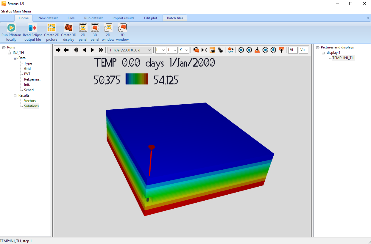
Launch Stratus and open the ECLIPSE restart file, INJ_TH.GRID. Create a Temperature 3D display, which soon after created will show the initial vertical temperature distribution:
Then advance in time until the last time step to see the temperature distribution at the end of the 7 years injection (Dec 2006):
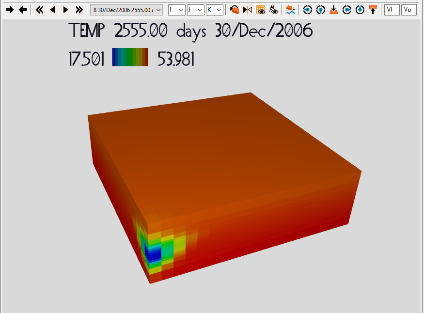
You can see that in the region around the injector the temperature has dropped to about 17 C.
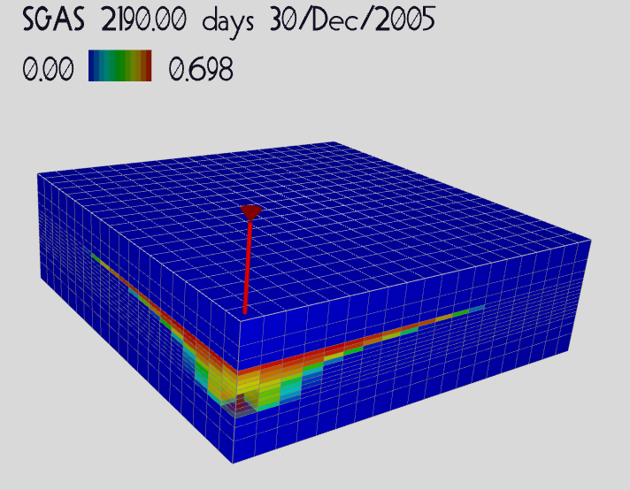
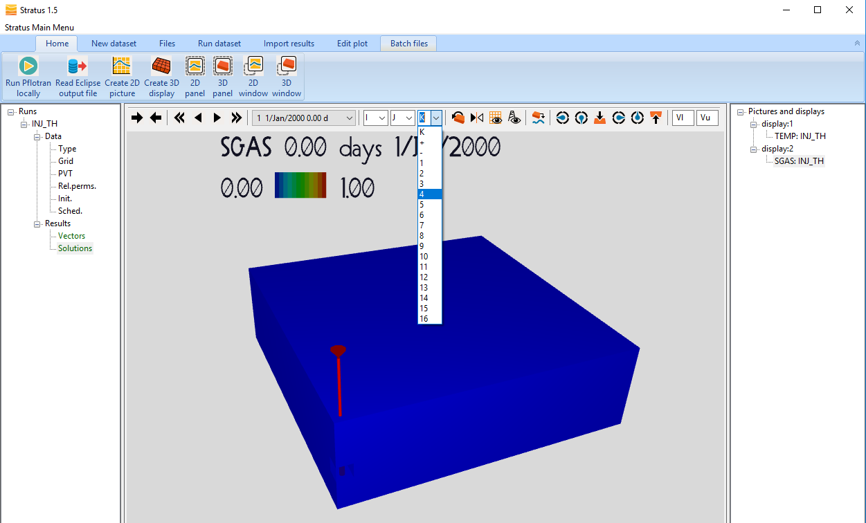
To display the gas saturation distribution create a new 3D display for SGAS. Then, to analyse how the gas spread below the caprock, create a horizontal slice at K=4 from the drop-down menu of the k slicing-filter:
At this point advance the time to analyse the CO2 migration:
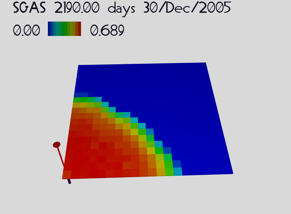
As expected, after 7 years of injection the CO2 has migrated upwards and spread under the caprock. The asymmetry observed is due to the permeability heterogeneity.
Analyse the well BHP and BHT
Click on Create 2D Picture (graph), select WBHP (well bottom hole pressure) and Add Line, then select WTEMP (well temperature) and Add line:
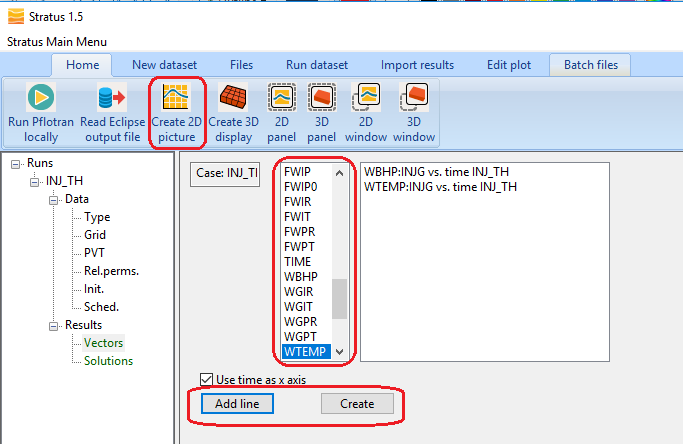
Then click on Create (next to Add line) to generate the 2D picture (graph). Select the 2D Picture (graph) on the right-side tree menu to display on the main panel:
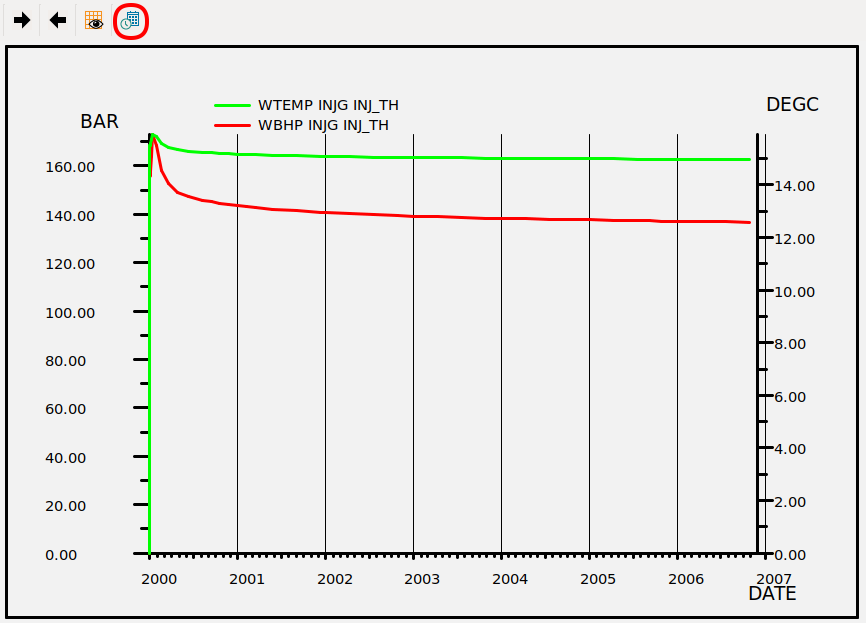
In the tool bar above the graph use the calendar/time icon to switch between the x-axis format from days to dates.
The BHP of the injector reaches ~170 Bar during the start-up, then decreases gradually to ~138 Bar. The temperature in the well borehole starts at 15.9 C and reduces to about 15 C at the end of the injection.
Analyse Temperature and properties in a grid block completed by the well
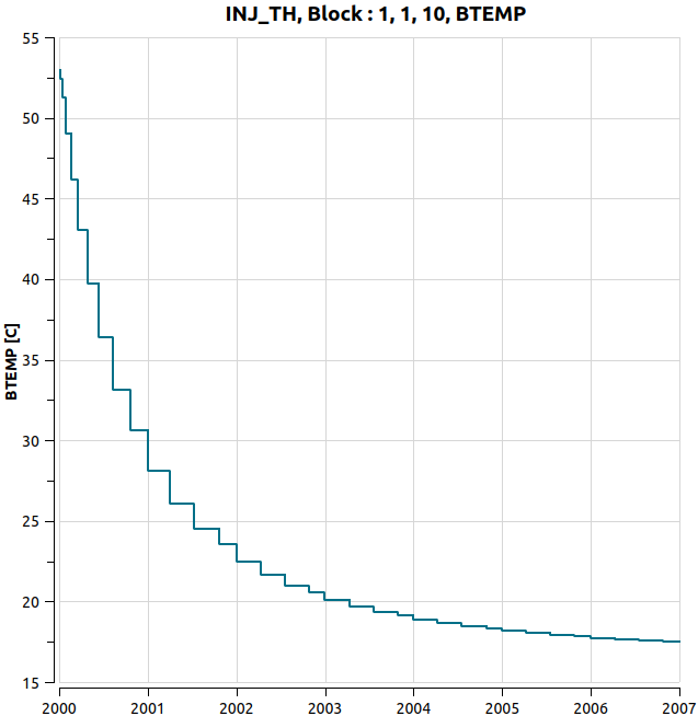
Click on Create 2D picture, select BTEMP and the block (1,1,10), which is one of those completed by the injector. Then Add Line and Create:
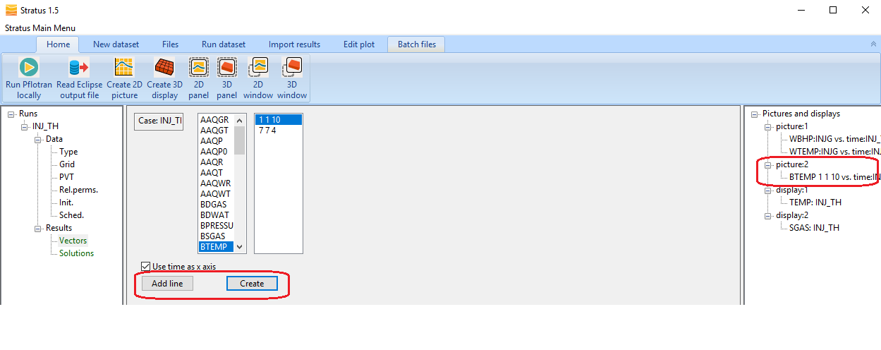
In the right-side tree menu select the BTEMP picture (graph) just created. This will show the temperature variation nearby the well during the injection:
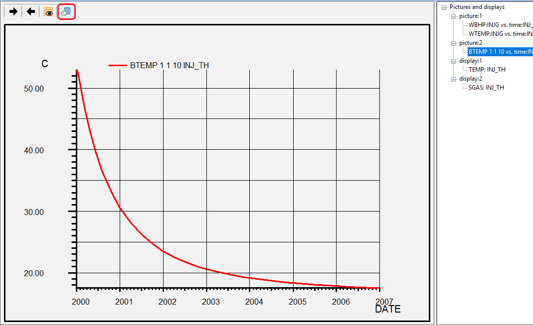
Use the calendar/time icon to switch the time axis format from days to dates. The temperature of the completed grid block (1,1,10) drops over time as CO2 is being injected. Following the same steps to create the temperature profile, you can create the gas density and viscosity plots in the same block. If you want to see more pictures (graphs) on multiple Windows, you can select a Picture (graph) from the right/side tree menu, and click on 2D Window. This will create a new 2D Window of the selected picture:
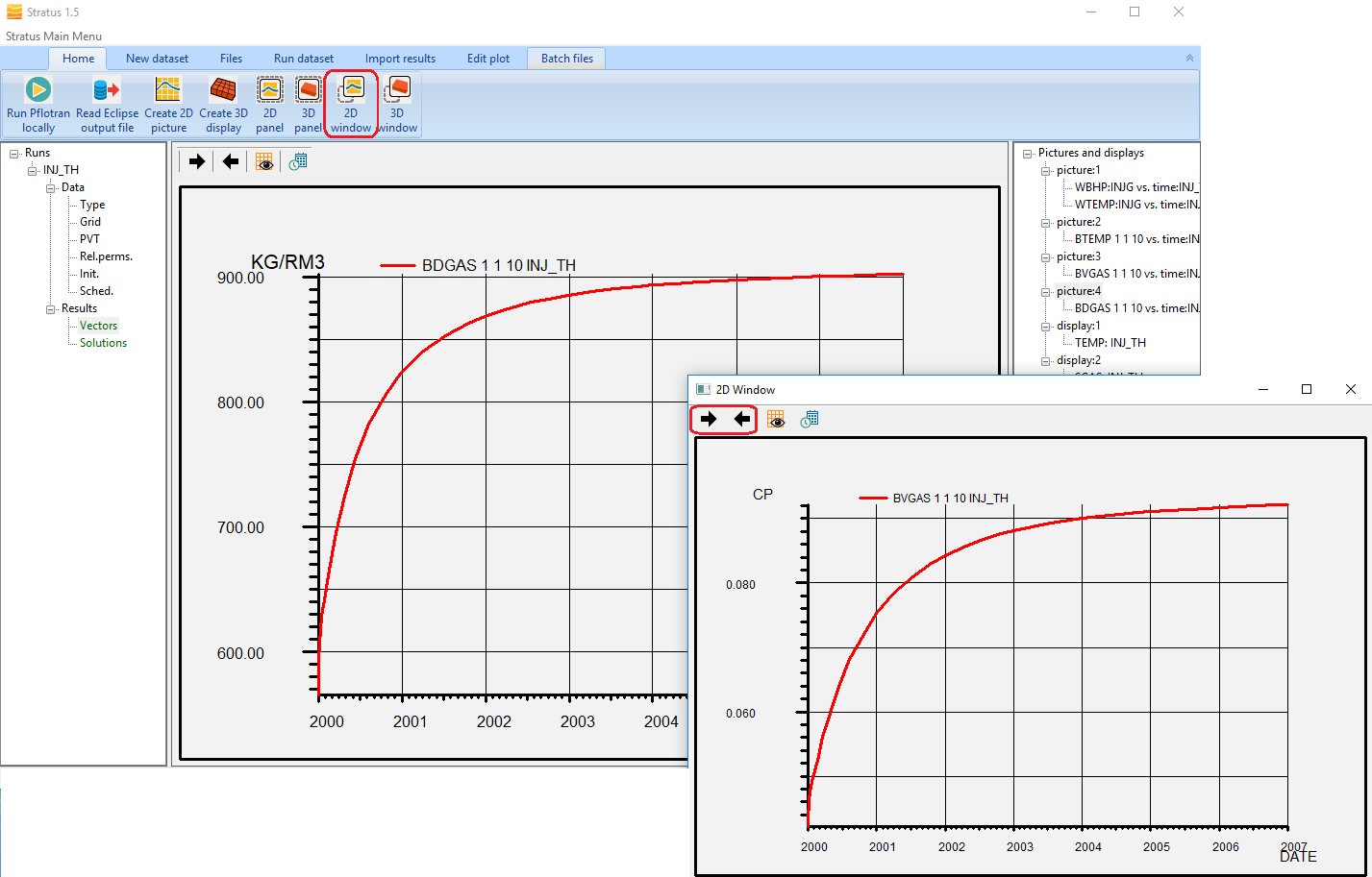
To change picture (graph) in a 2D window or in the 2D Panel, use the forward and backward black arrows on the top left corner. With these arrows you can browse all graphs previously created.
As expected, the CO2 viscosity and density increase significantly as the the temperature decreases.
Do not close the Stratus window, as you will load another run in the next section of this tutorial. To continue go to Set up a restart run and simulate the post injection phase.
Analyse the results of the thermal injection run with ResInsight
Visualise 3D Temperature and gas saturation
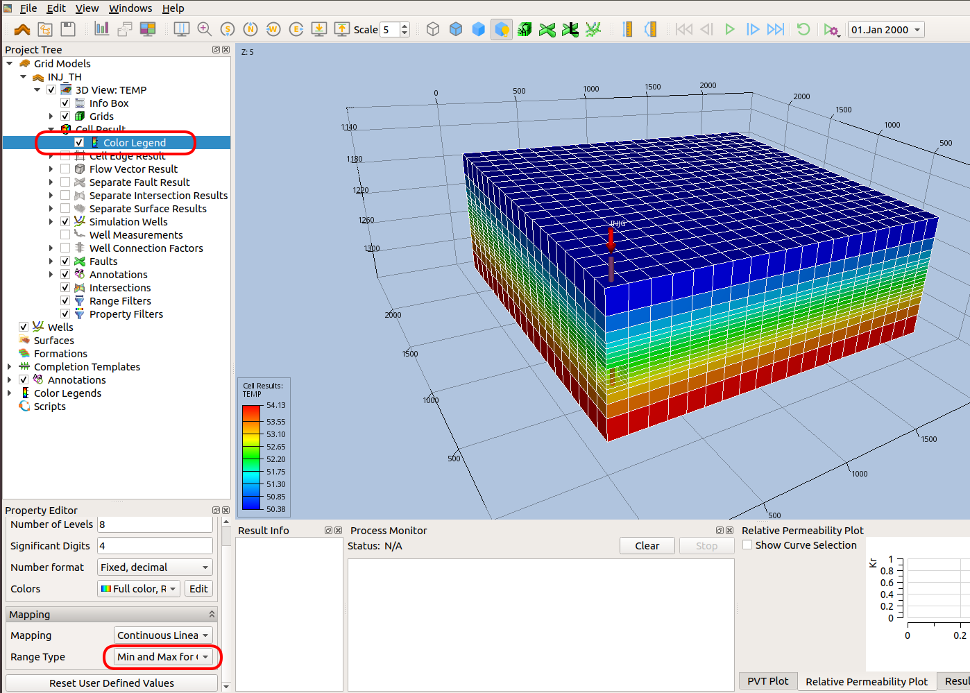
Launch ResInsight and open the ECLIPSE restart file, INJ_TH.GRID. Select Temperature from cell results. To see the initial vertical temperature distribution, select “Color Legend” in the Cell Result sub-menu, then on the bottom left corner, select “Min and Max for the current time step” in the Range Type drop-down menu:
Then advance the time until the last time step to see the temperature distribution at the end of the 7 year injection (Dec 2006):
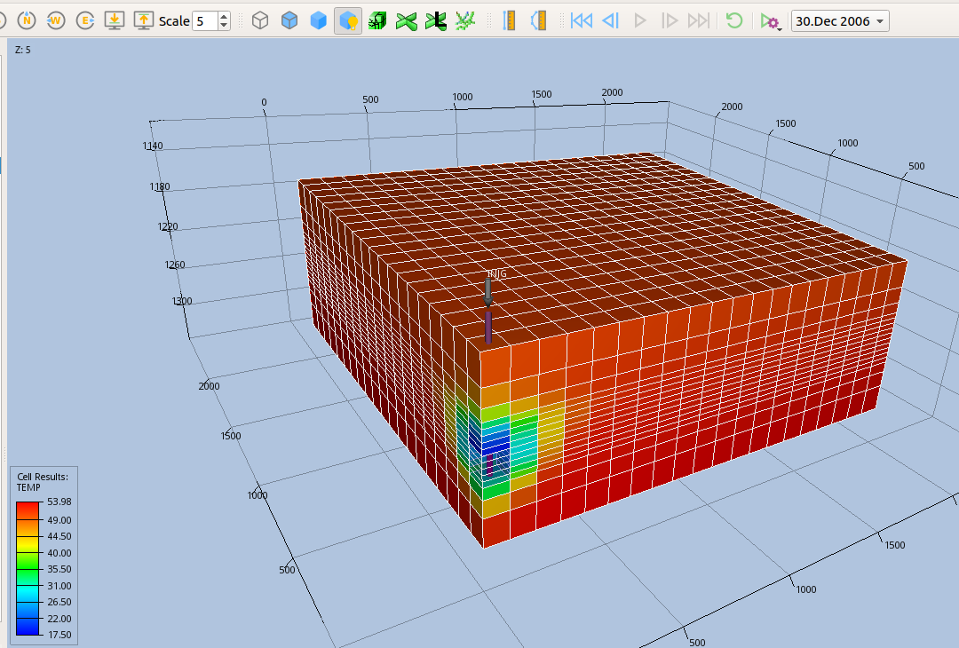
You can see that in the region around the injector the temperature has dropped to about 17 C.
To display the gas saturation distribution select SGAS from Cell Results. Then apply a K-range filter to see the gas saturation just below the caprock. To do this right-click “Cell Filters” in the left side menu, right-click and select “New range filter”. Then on the bottom left corner, enter 4 in the K Start box, and type enter.
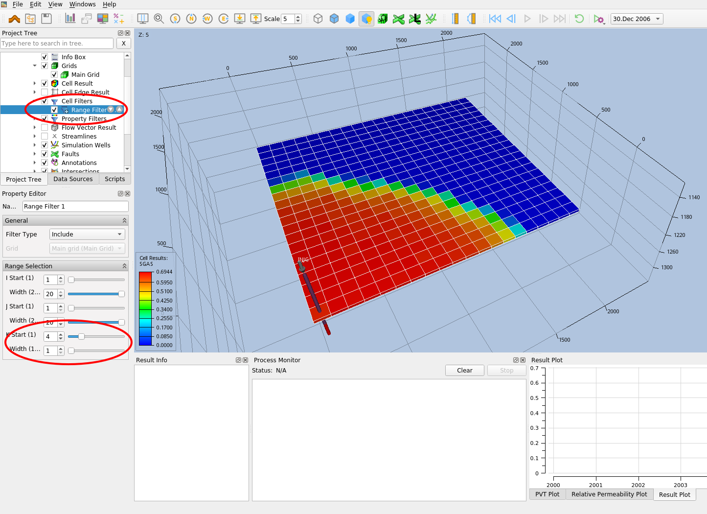
As expected, after 7 years of injection the CO2 has migrated upwards and spread under the caprock. The asymmetry observed is due to the permeability heterogeneity.
Analyse the well BHP and BHT
Click on the graph icon on the top left corner:
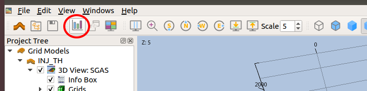
The line plots editors will open:
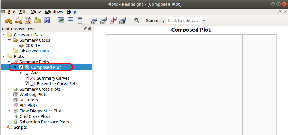
To display the curves available for plotting, right click on “Compose Plot”, and click on “Edit Summary Plot”. The following pop-up windows will open:
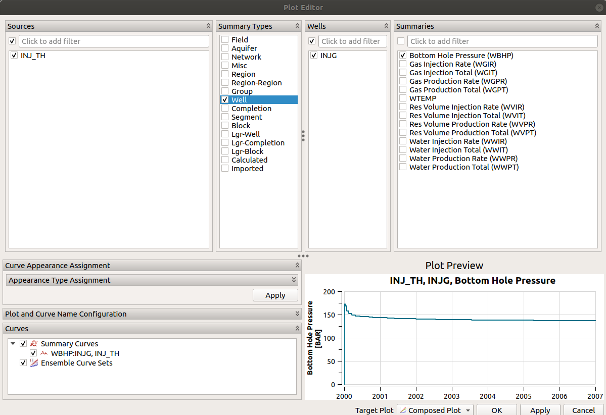
To plot the injector bottom hole pressure (BHP), from left to right select, INJ_TH, Well, INJG, WBHP. Then click Ok. Repeat for the bottom hole temperature (BHT), reported as WTEMP. Below are the two plots you will generate for BHP and BHT vs time:
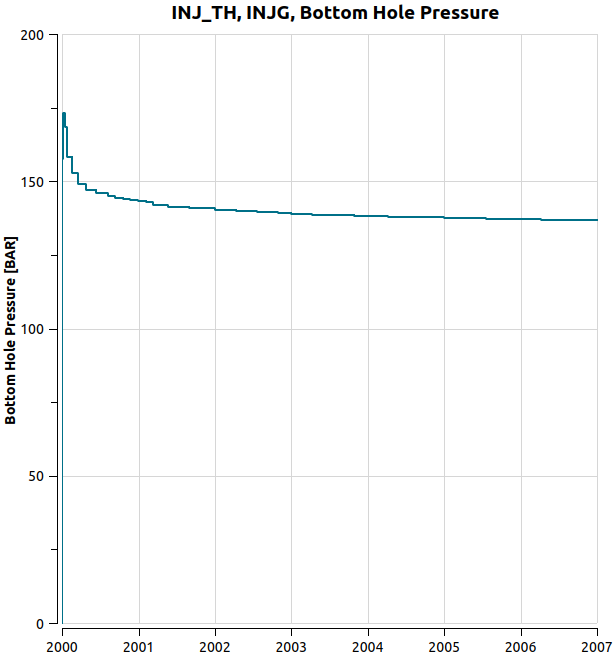
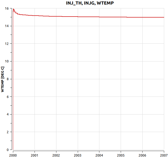
The BHP of the injector reaches ~170 Bar during the start-up, then decreases gradually to ~138 Bar. The temperature in the well borehole starts at 15.9 C and reduces to about 15 C at the end of the injection.
Analyse Temperature and properties in a grid block completed by the well
In the Plot Editor, right-click on Summary Plots, and select New Summary plot.
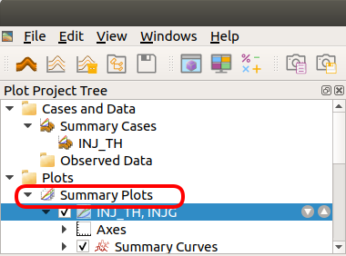
This will create a new Composed Plot under Summary Plots. Right-click on the new Composed Plot, and select “Edit Summary File Plot”. Then select the grid block viewer, grid block (1,1,10), and BTEMP:
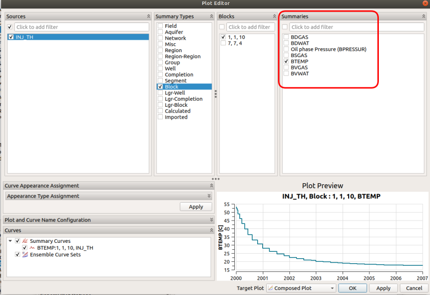
Click ok to see the plot of temperature vs time.
The temperature of the completed grid block (1,1,10) drops over time as CO2 is being injected. Following the same steps to create the temperature profile, you can create the gas density and viscosity plots:
As expected, the CO2 viscosity and density increase significantly as the the temperature decreases.
Do not close the ResInsight window, as you will load another run in the next section of this tutorial. To continue go to Set up a restart run and simulate the post injection phase.
Setup a restart run and simulate the post-injection phase
To continue the simulation after the injection, and assess the time needed for the reservoir to recover its initial temperature, you will create a new run that continues from the ECLIPSE restart file of the injection run (INJ_TH).
Open the input deck of the injection run (INJ_TH.in), and save it with a different file name (e.g. POST_INJ_TH.in) in the same folder.
Now define the restart file from which the post-injection run will restart to continue the simulation beyond the injection. At the end of the SIMULATION block add the ERESTART keyword, followed by the root name of the previous run, i.e. INJ_TH, and the restart time, i.e. 7 years:
SIMULATION
  SIMULATION_TYPE SUBSURFACE
  PROCESS_MODELS
    SUBSURFACE_FLOW Flow
      MODE GAS_WATER
      OPTIONS
        RESERVOIR_DEFAULTS
      /
    / ! end of subsurface_flow
  / ! end of process models
  ERESTART INJ_TH 7 y
END  !! end simulation block
With the instructions above, when running POST_INJ_TH.in, PFLOTRAN-OGS will look for the following three files in the same location where POST_INJ_TH.in is stored:
INJ_TH.UNRST
INJ_TH.UNSMRY
INJ_TH.SMSPEC
It will the scan these files searching for the time at year 7.
You will need to extend the simulation final time and tune the maximum time step constraints. Set the final time to 500 years, and a growing maximum time step: 1 year when the simulation reaches 3000 days (injection stop), and 1000 days when the simulation reaches 25 years.
TIME
  !uses default start date JAN 2000
  FINAL_TIME 500 y
  INITIAL_TIMESTEP_SIZE 0.1 d
  MAXIMUM_TIMESTEP_SIZE 100 d at 0 d
  MAXIMUM_TIMESTEP_SIZE 365 d at 3000 d
  MAXIMUM_TIMESTEP_SIZE 1000 d at 18250 d
END
The simulation will restart from 7 years, and carry on until 500 years. This is enough to see a temperature recovery.
Finally, ask for additional reporting times (10, 50, 100, 200, 300, 400, 500) in ECLIPSE_FILE to analyse the post injection phase.
OUTPUT
  MASS_BALANCE_FILE
   PERIODIC TIMESTEP 1
  END
  ECLIPSE_FILE
    TIMES y 1 2 3 4 5 6 7 10 50 100 200 300 400 500
    PERIOD_SUM TIMESTEP 1
    OUTFILE
    WRITE_DENSITY
    WRITE_VISCOSITY
    SUMMARY_D
      BPR   1  1  10
      [………………………………]
      BTEMP 7  7   4
    END_SUMMARY_D
  END
  LINEREPT
END
Run the simulation defined by POST_INJ_TH on your preferred environment. Open one of the links below on a new tab, so you can continue following the instructions to analyse the result in this page.
Analyse results of Post-Injection simulation
Continue this tutorial analysing the results using Stratus or ResInsight, clicking one of the links below:
Analyse the results of the thermal post-injection run with Stratus
Analyse the results of the thermal post-injection run with ResInsight
Analyse the results of thermal post-injection run with Stratus
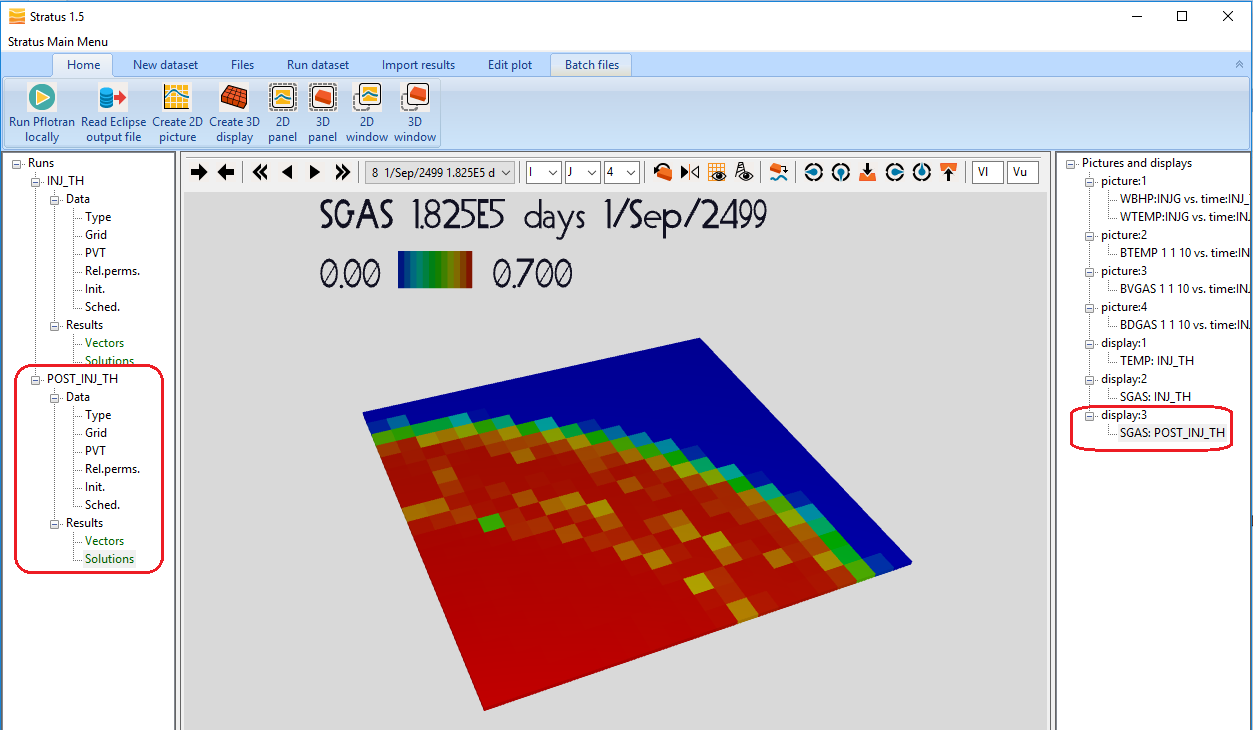
Assuming you still have Stratus open with the INJ_TH run executed earlier, import also the ECLIPSE files for the POST_INJ_TH case, to have both runs loaded. Once you have done this, you will see both runs on the left-side menu. To visualise the gas saturation evolution under the caprock during the post-injection phase, create a 3D Display of SGAS for the POST_INJ_TH run. Then select a horizontal slice setting K=4:
As you advance the time, you will see that the gas plume grows significantly until 2100 (i.e. during the first 100 years), it then starts shrinking slowly as the CO2 dissolution into the underlying brine proceeds.
To analyse how the temperature changes around the injector combining the results of the two runs, click Create 2D picture, and for each run select BTEMP, grid block (1,1,10), and click Add line:
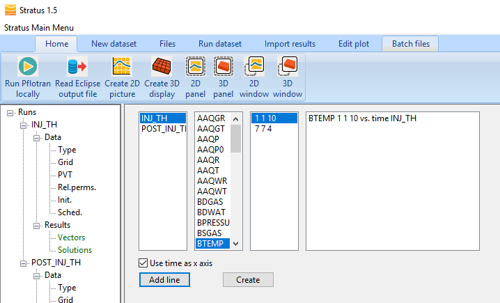
Once you have added the BTEMP lines from both runs, click Create, and select the Picture you just created from the right-side tree menu:
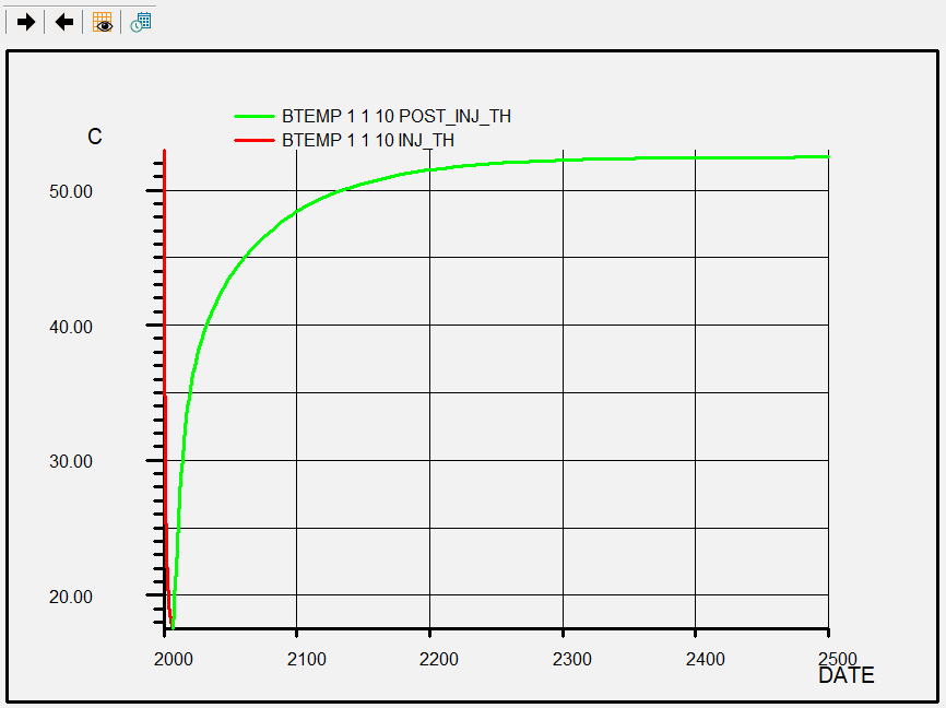
This plot shows temperature vs time in the block (1,1,10) from 1 to 7 years (2000-2007) from the INJ_TH run, and from 7 to 500 years (2007-2500) from the POST_INJ_TH run. After 200 years, the temperature in the grid block (1,1,10) completed by the injector has nearly recovered the value it had before the cold injection.
Analyse the results of thermal post-injection run with ResInsight
Assuming you still have ResInsight open with the INJ_TH run executed earlier, import also the ECLIPSE files for the POST_INJ_TH run, to have both runs loaded. Once you have done this, you will see both runs on the left-side menu. To visualise the gas saturation evolution under the caprock during the post-injection phase, select SGAS from Cell Results for the POST_INJ_TH run. Then create a “New K-slice range filter” and set K=4:
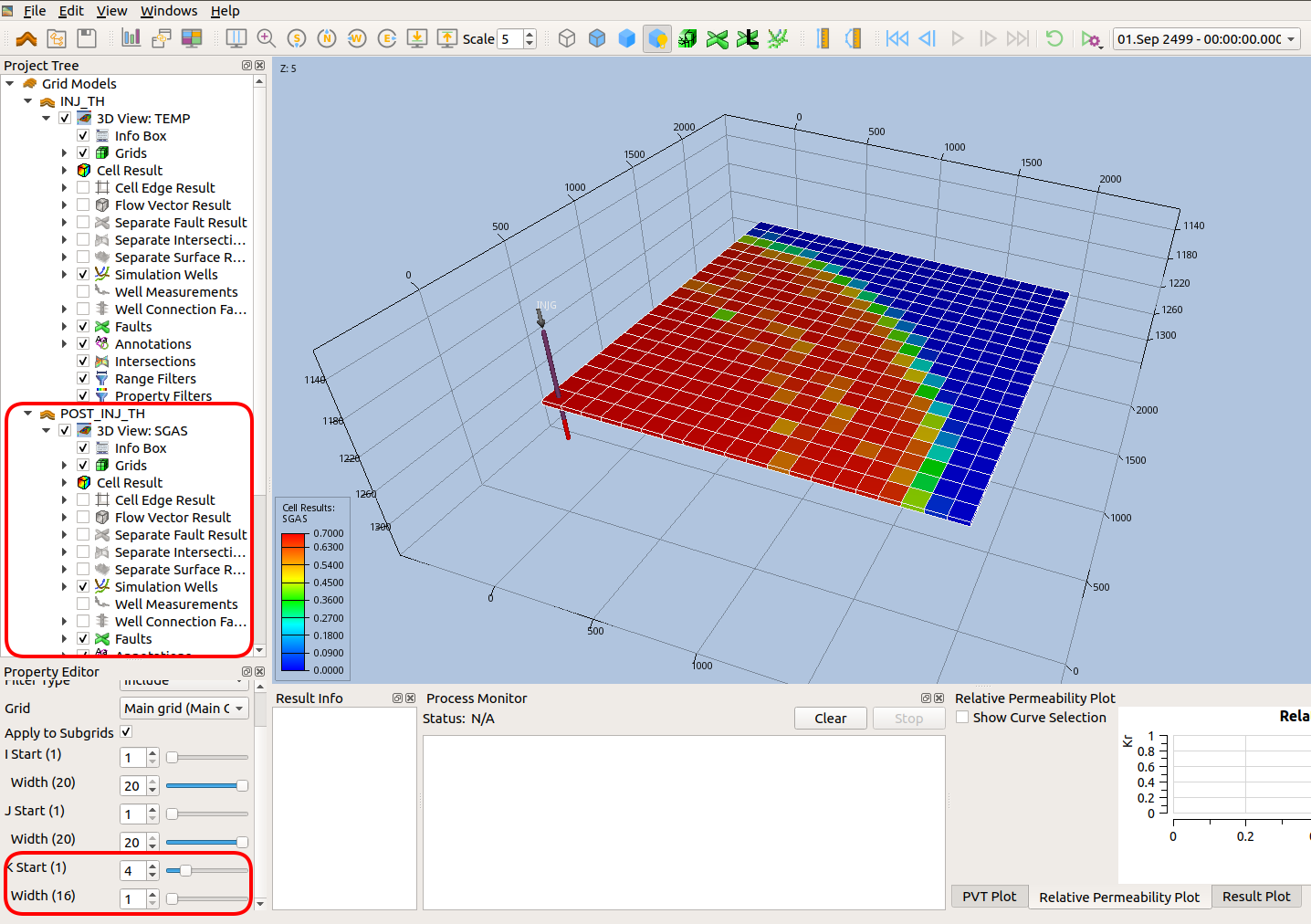
As you advance the time, you will see that the gas plume grows significantly until 2100 (i.e. during the first 100 years), it then start shrinking slowly as the CO2 dissolution into the underlying brine proceeds.
To analyse how the temperature changes around the injector, open the Plot Window. In the Plot Project tree scroll down until you find the summary plot you generated earlier for the temperature vs time in the grid block (1,1,10). Then right click and select Edit Summary plot. In the window that will open, do the following selection to see the temperature plot in the grid block (1,1,10) from both runs:
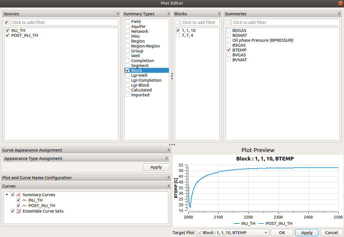
Click ok, and you will obtain a plot of temperature vs time in the block (1,1,10) from 1 to 7 years (2000-2007) from the INJ_TH run, and from 7 to 500 years (2007-2500) from the POST_INJ_TH run:
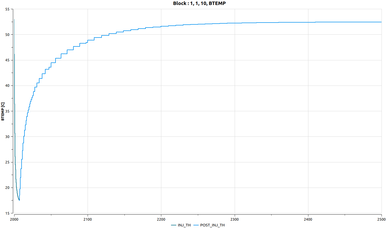
After 200 years, the temperature in the grid block (1,1,10) completed by the injector has nearly recovered the value it had before the cold injection.