Tutorial 3 – CO2 Storage sites connected to a nearby hydrocarbon field
You will learn about:
setting up a model using a reservoir geometry and geology given in ECLIPSE format
setting up relative permeability hysteresis
using calendar dates to define simulation events
setting up horizontal wells
To run this tutorial you will need the following:
Nine input files are used for this tutorial, these can be downloaded at the following links:
These are available as a zip file:
In addition you will need:
Stratus or ResInsight installed in your local machine
Tutorial sections:
Problem description
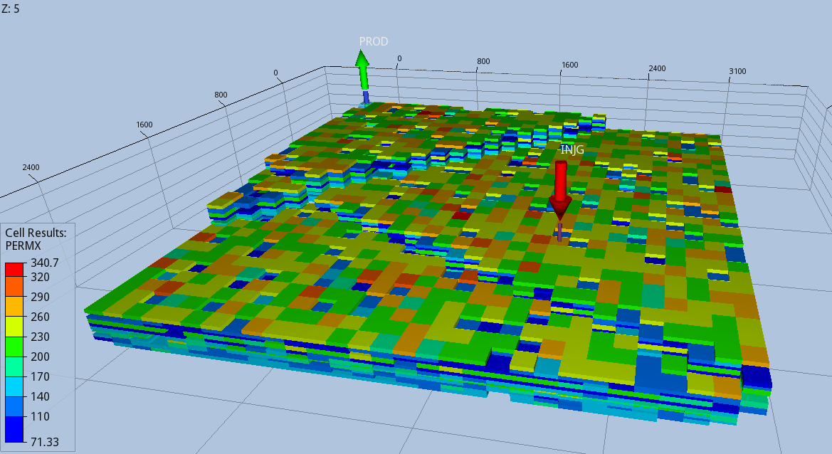
This tutorial describes a CO2 storage problem into a saline aquifer in proximity of a hydrocarbon field. As the two are pressure-connected, the depletion of the hydrocarbon field causes a pressure gradient that drives the CO2 plume migration. The depletion of the hydrocarbon field is modelled using a dummy well producing brine. The storage layer is split in two compartments by a fault, which is crossed by the CO2 plume during the post-injection migration phase.
The target layer extends 3 km x 3 km in the horizontal directions, and has a thickness of about 100 meters.
Setup of the input file
With a text editor open the input deck provided for this tutorial, CCS_3DF.in. The explanation below discuss only sections with instructions not covered in Tutorial 1.
Simulation – Hysteresis and STRAND set up
You switch on the hysteresis modelling adding the HYSTERESIS keyword in the OPTIONS of the GAS_WATER mode in the SIMULATION block:
SIMULATION
  SIMULATION_TYPE SUBSURFACE
  PROCESS_MODELS
    SUBSURFACE_FLOW Flow
      MODE GAS_WATER
      OPTIONS
       RESERVOIR_DEFAULTS
       ISOTHERMAL
       HYSTERESIS
       STRAND
      /
    /
  /
END
HYSTERESIS switches on the relative permeability hysteresis modelling for both non-wetting and wetting phases, which are the gas and brine in this case. In addition to the drainage saturation functions, PFLOTRAN-OGS expects also imbibition curves for both the aqueous and gas phases. If the imbibition curves are provided only for the gas phase, no hysteresis model will be applied to the brine relative permeability.
Both drainage and imbibition saturation functions are supplied in CHARACTERISTIC_CURVES.
When asking for HYSTERESIS, the user must also supply two indices for each grid block, one for the drainage function and the other for the imbibition curve. These are provided in the grdelc file by the SATNUM and IMBNUM arrays.
The keyword STRAND is also present under the SIMULATION block, which tells the simulator to output a report of stranded gas to the summary file.
Grid
You must define the simulation grid and its static properties (permeabilities, porosities, etc.) by an include file in the grid block:
GRID
  TYPE grdecl ccs_3df.grdecl
END
This the ccs_3df.grdecl file provided with this tutorial, which you can open with a text editor:
DIMENS
30 30 12 /

external_file ccs_3df_geom.grdecl

external_file ccs_3df_prop.grdecl

EQUALS
 ACTNUM 0 7 7 15 15 1 1
 ACTNUM 0 30 30 29 29 12 12
/

EQUALS
SATNUM 1     /
IMBNUM 2    /
/
The instructions describe a grid of 10800 blocks, with their locations defined by the coordinates of their corner points, provided in the include file “ccs_3df_geom.grdecl”, and their static properties (porosity and permeability) given in the other include file “ccs_3df_prop.grdecl”. These two files follow the format of a GRDECL Grid, as any other input card defined in ccs_3df.grdecl.
Following the GRDECL Grid convention, you can set the porosity or ACTNUM to zero for the cells you want to deactivate – the grid above use both methods. Inactive cells do not take part of the fluid flow computation, saving memory and computational resources.
All entries of the SATNUM array are assigned to 1, which means the first set of characteristic curves (saturation functions) found in the input deck will be used by each grid block for the drainage process.
All entries of the IMBNUM array are assigned to 2, which means the second set of characteristic curves (saturation functions) found in the input deck will be used by each grid block for the imbibition process (re-wetting).
Characteristic Curves
You define two set of characteristic curves (saturation function), one for the drainage and the other for the imbibition process. Note that the order these are entered is important, the first set of curves automatically take the integer id 1, the second the integer id 2. These integer ids are used by the SATNUM and IMBNUM arrays to assign saturation functions to each grid block.
!id=1
CHARACTERISTIC_CURVES drainage
 TABLE swfn_table
   PRESSURE_UNITS Bar
   external_file SWFN_drain.dat
 END
 TABLE sgfn_table
  PRESSURE_UNITS Bar
   external_file SGFN_drain.dat
 END
/

!id=2
CHARACTERISTIC_CURVES imbibition
 TABLE swfn_table
   PRESSURE_UNITS Bar
   external_file SWFN_imb.dat
 END
 TABLE sgfn_table
  PRESSURE_UNITS Bar
   external_file SGFN_imb.dat
 END
/
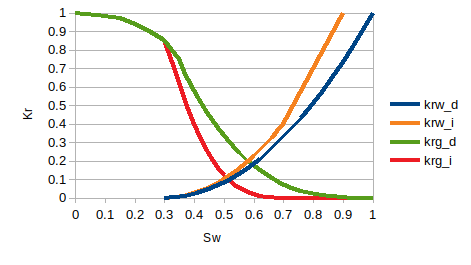
The SWFN and SGFN table for each set are provided by include files provided with this tutorial. If you plot the curves provided in the include files, you can see the shape and end points of the drainage and imbibition relative permeabilities:
Time
In the time block you can use calendar dates to define the start and end of the simulation. In this tutorial a 200 years simulation is set up, starting from 1 JAN 2025:
TIME
  START_DATE 1 JAN 2025
  FINAL_DATE 1 JAN 2225  ! 200 years simulation
  INITIAL_TIMESTEP_SIZE 1 d
  MAXIMUM_TIMESTEP_SIZE 30 d at 0. d
  MAXIMUM_TIMESTEP_SIZE 1 y at 10 y
END
Output
Ask for a solution report every 20 time steps and for key events such as the start and stop of CO2 injection, the stop of hydrocarbon production and the simulation end.
OUTPUT
  MASS_BALANCE_FILE
   PERIODIC TIMESTEP 1
  END
  ECLIPSE_FILE
    PERIOD_SUM TIMESTEP 5
    PERIOD_RST TIMESTEP 20
    WRITE_DENSITY
    WRITE_RELPERM
    DATES 1 JAN 2027 ! CO2 injection starts
    DATES 1 JAN 2031 ! CO2 injection stops
    DATES 1 JAN 2033 ! Production stops
    DATES 1 JAN 2225 ! Simulation ends
    OUTFILE
  END
  LINEREPT
END
Ask the simulator to output relative permeability in the restart files, by inserting WRITE_RELPERM in the ELCIPSE_FILE block. The analysis of relative permeability can be useful when modelling hysteresis.
Wells
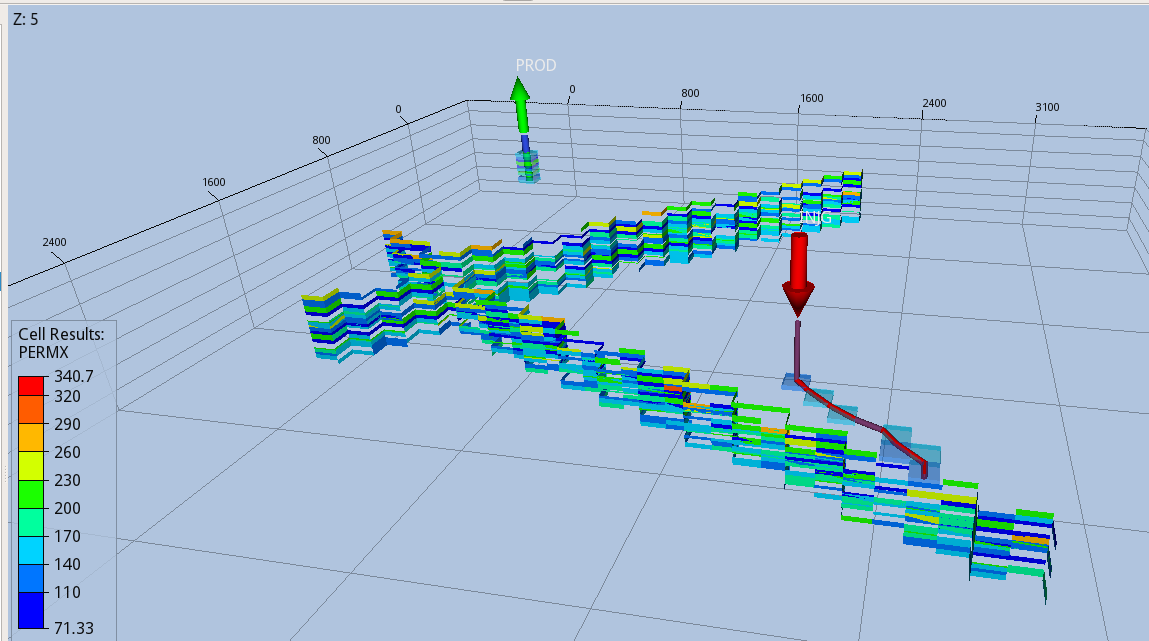
Define the horizontal CO2 injector by including completed grid blocks one by one, and specifying the drilling direction as X. There are 8 completions, all in the layer above the bottom one. The injector is shut during the first 2 years, it then opens on 1 JAN 2027 with a target mass rate of 0.682 Mt/year, and shuts on 1 JAN 2031.
WELL_DATA injg
  CIJK_D 21 21 11 11
  CIJK_D 22 22 11 11
  CIJK_D 23 23 11 11
  CIJK_D 24 24 11 11
  CIJK_D 24 25 11 11
  CIJK_D 25 25 11 11
  CIJK_D 25 26 11 11
  CIJK_D 26 26 11 11
  CONST_DRILL_DIR DIR_X
  DIAMETER 0.1524 m
  WELL_TYPE GAS_INJECTOR
  BHPL     400    Bar
  SHUT
  DATE 1 JAN 2027            ! Open injector 2 years after simulation starts
  OPEN
  TARG_GM 0.682 Mt/y
  DATE 1 JAN 2031            ! Shut well 4 years after injection started
  SHUT
END
Add the brine producer that models the pressure depletion caused by the nearby hydrocarbon field. This is vertical and located at the opposite corner of the injector, in the other side of the fault. Production occurs since the start of the simulation and lasts 8 years until 1 JAN 2033.
WELL_DATA prod
  CIJK_D 1 1 1 12
  DIAMETER 0.1524 m
  WELL_TYPE PRODUCER
  BHPL      150 Bar
  TARG_WSV  1000 m^3/day
  DATE 1 JAN 2033            ! Close producer 8 years after simulation starts
  SHUT
END
Below is a representation of the wells.
Run the simulation
Run the simulation set up for this tutorial on your preferred environment. Open one of the links below on a new tab, so you can continue following the instructions to analyse the result in this page.
Analyse the results
The simulator outputs the ECLIPSE restart and summary files (CCS_3DF.UNRST, CCS_3DF.UNSMRY, CCS_3DF.SMSPEC), which you can load with any post-processor supporting this format.
Continue this tutorial analysing the results using Stratus or ResInsight, clicking one of the links below:
Analyse the results of the CCS_3DF run with Stratus
Launch Stratus, and load the “CCS_3DF.GRID” file. Then plot the field average pressure, and using the Edit Line Plots setting adjust the time range to display the period from 2025 to 2035, (i.e. the first 10 years of simulation). This can be done entering 4000 days as the maximum value for the x-axis:
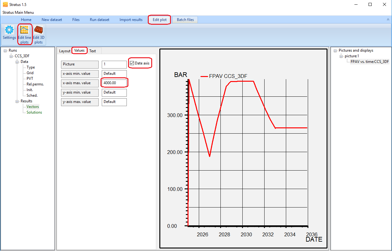
To display the graph on the whole panel, leave Edit Line Plots by clicking on picture1 on the right-side tree menu,
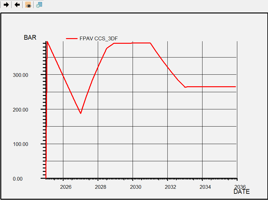
FPAV shows a pressure drop from 400 to 200 Bar caused by the hydrocarbon depletion during the first two yeas. At this point the CO2 injection starts, and the reservoir starts recovering the pressure until the injector reaches its BHP limit (400 Bar). In 2031 the injector is shut, while the producer keeps depleting the reservoir until Jan 2033, bringing the pressure down again to about 260 Bar.
Now create a 3D display of SGAS, and advance the time to the end of the simulation (2225):
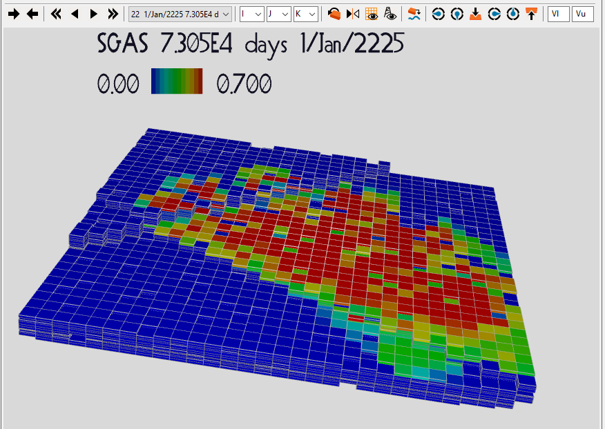
During the post-injection the CO2 migrates towards the shallower low-pressure region around the producer.
To analyse the effect of the hysteresis create a slice for I = 22, and select the grid block (22,22,5), above the injector:
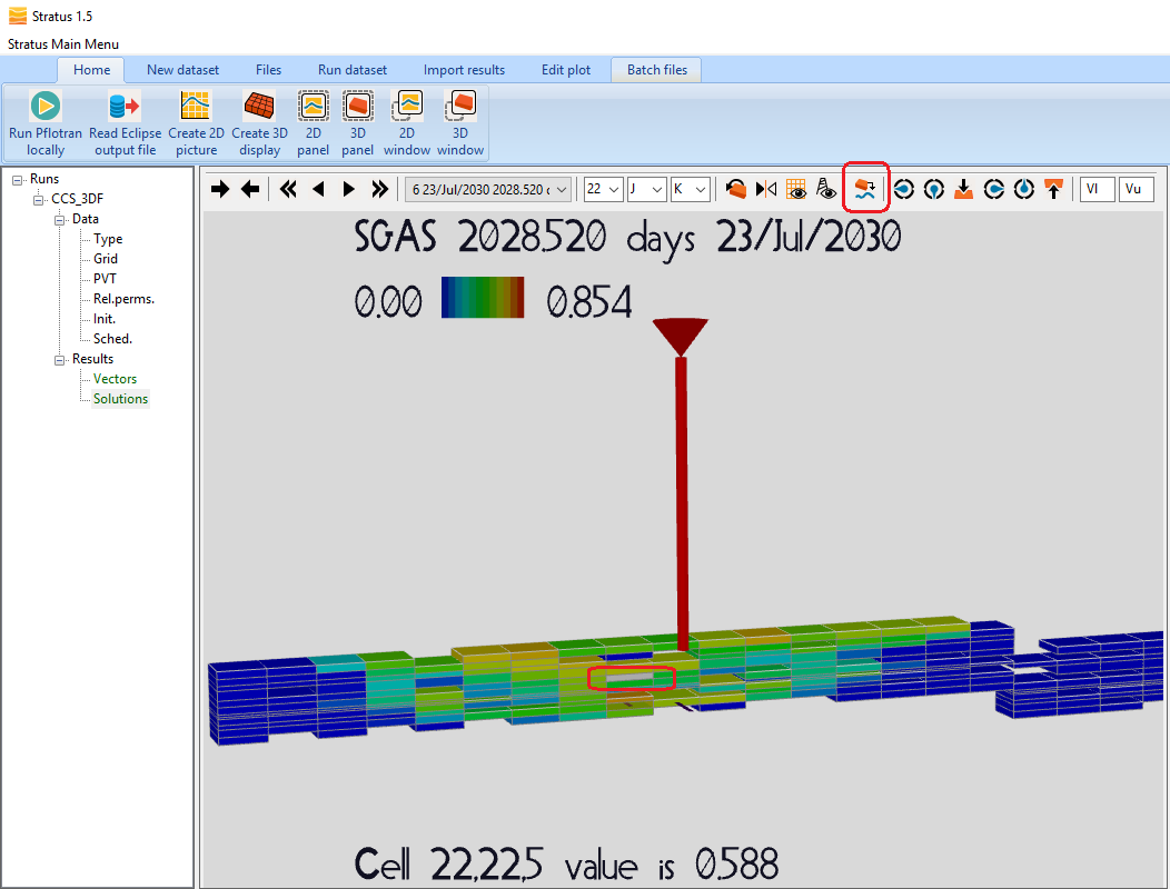
Click on the Plot wrt time icon (highlighted by a red circle above), which will create a plot of SGAS vs time for the selected grid block:
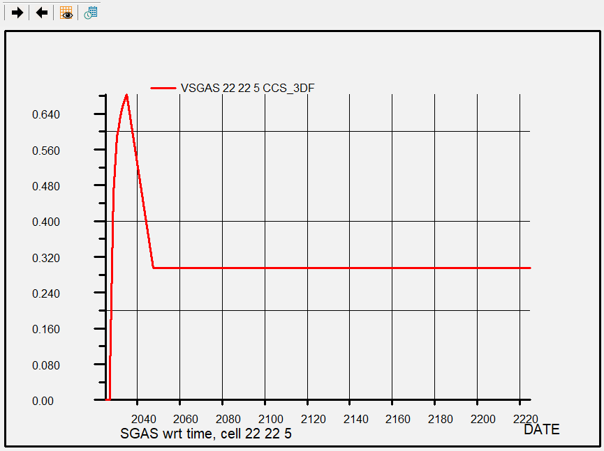
The gas saturation grows until Nov 2034 (~ 2 years after the injection), due to the invasion of CO2 coming from the deeper layers completed by the injector. It then reduces as CO2 migrates towards the shallower layers, however the values does not drop below 0.3 as imposed by the imbibition curve that models the residual trapping.
Analyse the results of the CCS_3DF run with ResInsight
Launch ResInsight, and load the “CCS_3DF.GRID” file. Then plot the field average pressure, and using the Plot Axis setting adjust the time range to display the period from Jan 2024 to Jan 2035, (i.e. the first 10 years of simulation):
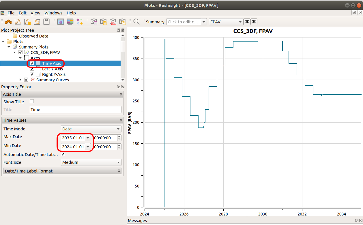
FPAV shows a pressure drop from 400 to 200 Bar caused by the hydrocarbon depletion during the first two yeas. At this point the CO2 injection starts, and the reservoir starts recovering the pressure until the injector reaches its BHP limit (400 Bar). In 2031 the injector is shut, while the producer keeps depleting the reservoir until Jan 2033, bringing the pressure down again to about 260 Bar.
Now click again on “Cell Result” on the left-side menu, and select gas saturation (SGAS) in the property editor. Advance the time to the end of the simulation (1 JAN 2225):
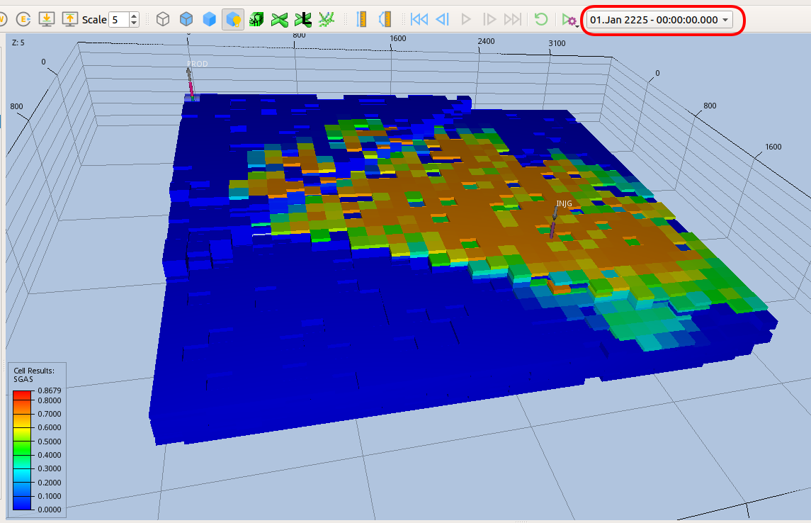
During the post-injection the CO2 migrates towards the shallower low-pressure region around the producer.
To analyse the effect of the hysteresis create a slice for I = 22, and select the grid block (22,22,5), above the injector:
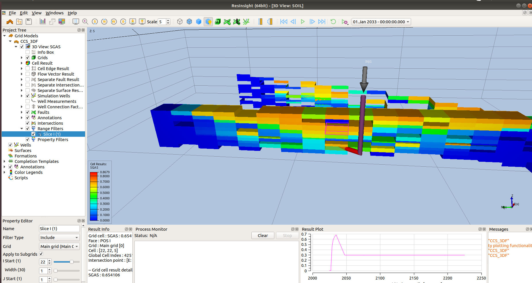
Right click and select Plot Time History For The Selected Cell, select Create New Plot, and click ok:
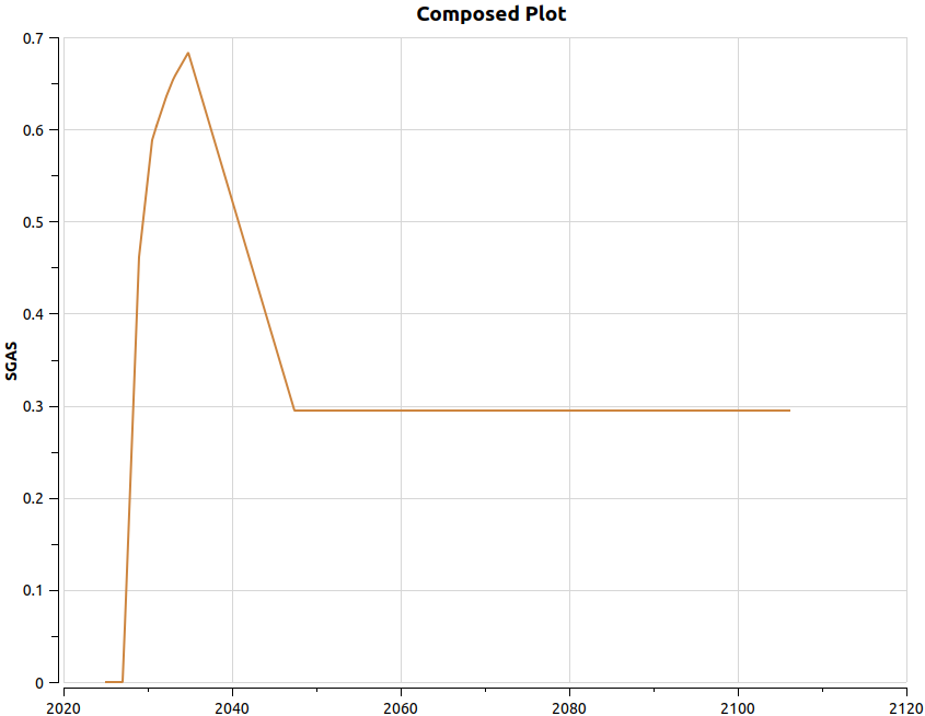
The gas saturation grows until Nov 2034 (~ 2 years after the injection), due to the invasion of CO2 coming from the deeper layers completed by the injector. It then reduces as CO2 migrates towards the shallower layers, however the values does not drop below 0.3 as imposed by the imbibition curve that models the residual trapping.