Tutorial 4 – CO2 Storage Into Depleted Gas Fields
You will learn about:
setting up a model for CO2 storage in a depleted gas field using the Multi-Gas model (COMP3)
analysing results of Multi-Gas models
To run this tutorial you will need the following:
Five input files are used for this tutorial, these can be downloaded at the following links:
These are also available as zip file:
In addition you will need:
Stratus or ResInsight installed in your local machine
Tutorial sections:
Problem Description
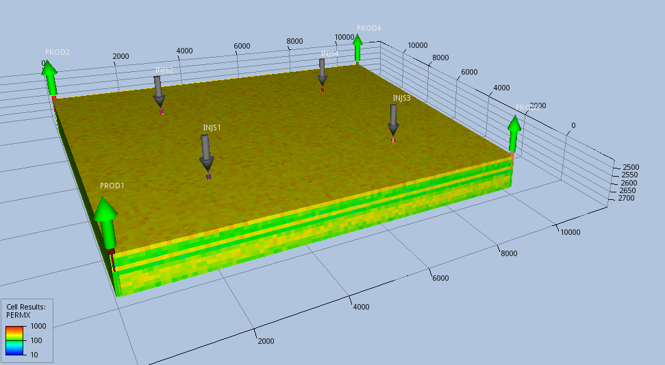
This tutorial describes a CO2 storage problem in a depleted gas field. The model is a reservoir layer initially filled with gas at about 300 Bar, covering a 10 km x 10 km area, from a depth of 2500 m to 2700 m, and discretised with 100,000 cells (a 100x100x10 regular grid). It is depleted using four corner wells for 15 years, starting from the beginning of 2010. Then four solvent (CO2) injectors are turned on in January 2025 and the reservoir is partially repressurised to a further 15 years. In 2040, after 15 years of CO2 injection, the wells are turned off and the reservoir is left to soak for a further 20 years until 2060.
Simulation – COMP3 setup
The problem is modelled with the isothermal Multi-Gas model, using the COMP3 mode, which models three components: water, reservoir gas and solvent (CO2). Select COMP3 in the SIMULATION block by using the MODE keyword:
SIMULATION
  SIMULATION_TYPE SUBSURFACE
  PROCESS_MODELS
    SUBSURFACE_FLOW Flow
      MODE COMP3
      OPTIONS
       ISOTHERMAL
       RESERVOIR_DEFAULTS
      /
    / ! end of subsurface_flow
  / ! end of process models
END  !! end simulation block
Setup of the input file
With a text editor open the input deck provided for this tutorial, DEP_GAS.in. The explanation below discuss only sections with instructions not covered in Tutorial 1 and Tutorial 3.
PVT and fluid properties
For the water, specify only the surface density, required by the simulator to compute fluid in place and surface volumes, and leave default internal correlations (IFC67) for the other properties. Define solvent as pure CO2 by including the external database generated by the Span and Wagner EOS. For the reservoir gas enter a user-defined PVDG table as the one provided in the input sample.
EOS WATER
  SURFACE_DENSITY 995.5
END

EOS GAS
  FORMULA_WEIGHT 16.04d0
  SURFACE_DENSITY 1.0995 kg/m^3
  PVDG
    DATA_UNITS ! Metric in the Eclipse sense
      PRESSURE  Bar
      FVF       m^3/m^3
      VISCOSITY cP
    END
    DATA
      TEMPERATURE 15.0
         1.0135  1.186979 0.0107
        34.4738  0.033261 0.0127
        68.9476  0.016001 0.0134
        82.7371  0.013160 0.0138
        103.421  0.010358 0.0145
        124.105  0.008535 0.0153
        137.895  0.007636 0.0159
        158.717  0.006597 0.0170
        172.369  0.006190 0.0177
        206.843  0.005531 0.0195
        241.317  0.005118 0.0214
        275.790  0.004840 0.0232
        310.264  0.004617 0.0250
        330.948  0.004509 0.0261
      END !end TEMP block
    END !endDATA
    !specify temperature dependency for viscosity
  END !end PVDG
END

EOS SOLVENT
  SURFACE_DENSITY 1.0 kg/m^3
  CO2_DATABASE co2_dbase.dat
END
Since the solvent is defined as CO2, by default the code uses the Duan & Sun correlation [DS03] to account for the CO2 dissolution in brine.
Equilibration
Set up the gas-water contact (WGC) below the reservoir, with a capillary pressure between gas and water at the WGC depth equal to zero. In this way only the gas cap will be modelled. Set the datum depth at the top of the layer (2500 m), imposing a pressure of 300 Bar:
EQUILIBRATION

  PRESSURE 300 Bar
  DATUM_D  2500 m
  WGC_D    2700.0 m
  PCWG_WGC 0.0    Bar

  RTEMP 139 C
/
Wells
The model has 4 corner producers and 4 solvent (CO2) injectors equally spaced, located 2.4 km away from the model boundaries. The producers shut in 2025, when the injectors open. The CO2 injection carries on for 15 years until 2040, after which the injectors are also shut. Below is a sample of the settings you require for one injector and one producer, all the others follow the same pattern:
WELL_DATA injs1
  RADIUS 0.0762 m
  CIJK_D 25 25 1 5
  WELL_TYPE SOLVENT_INJECTOR
  BHPL   500  Bar
  SHUT
  DATE 1 JAN 2025
  OPEN
  TARG_SSV 5000000 m^3/day
  DATE 1 JAN 2040
  SHUT
END

WELL_DATA prod1
  CIJK_D  1 1 5 10
  WELL_TYPE PRODUCER
  BHPL      50   Bar
  TARG_GSV 12000000 m^3/day
  DATE 1 JAN 2025
  SHUT
END
Run the simulation
Run the simulation set up for this tutorial on your preferred environment. Open one of the links below on a new tab, so you can continue following the instructions to analyse the result in this page.
Analyse the results
The simulator outputs the ECLIPSE restart and summary files (DEP_GAS.UNRST, DEP_GAS.UNSMRY, DEP_GAS.SMSPEC), which you can load with any post-processor supporting this format.
Continue this tutorial analysing the results using Stratus or ResInsight, clicking one of the links below:
Analyse the results of the DEP_GAS run with Stratus
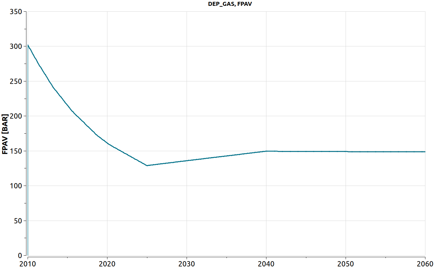
Launch Stratus, and load the “DEP_GAS.GRID” file. Then plot the field average pressure, and switch to the date format for the x-axis:
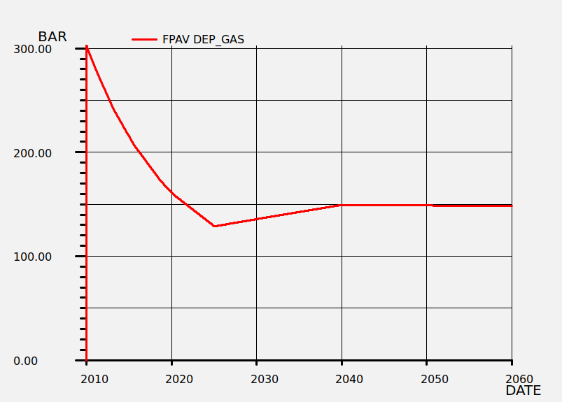
During depletion the pressure drops from 300 Bar to about 130 Bar, then it recovers to 150 Bars with the injection of CO2, and remain stable until the end of the simulation.
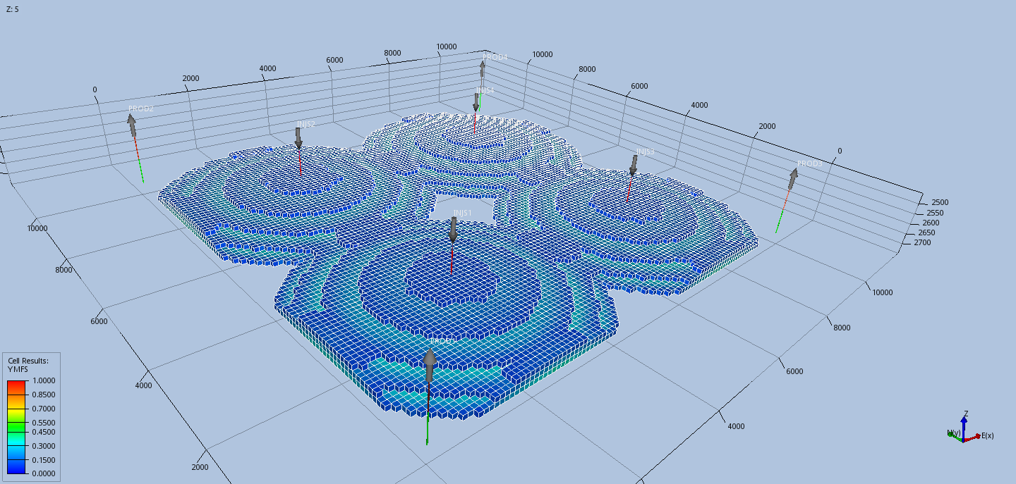
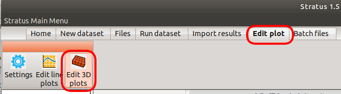
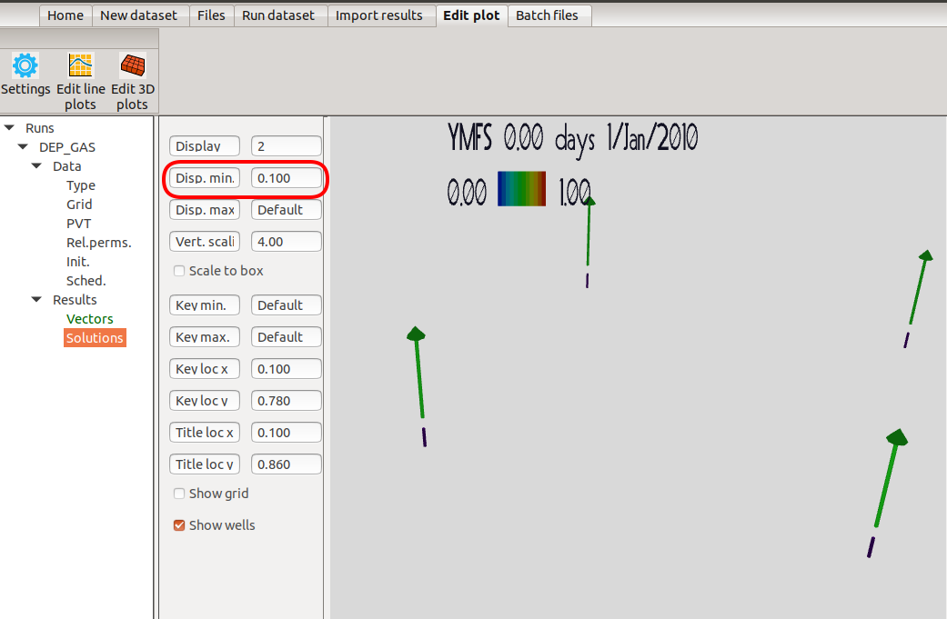
From Solutions in the left-side tree menu, create a 3D plot for the molar fraction of solvent in the vapour phase (YMFS). Then click on the “Edit 3D Plot”:
In the “Disp. Min” box, set the minimum threshold of YMFS, below which the 3D contour display will be cut:
Now click again over the YMFS 3D display you just created in the right-side tree menu, and advance the time until the end of the injection (1 Jan 2040):
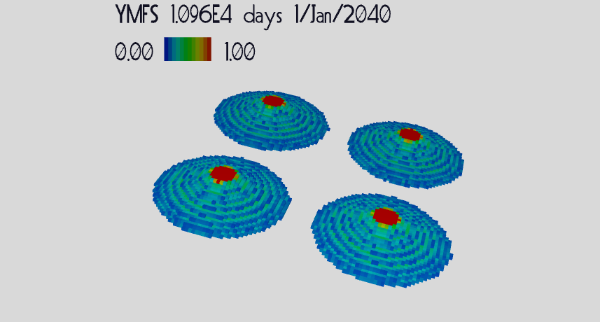
The plots above show how the CO2, being heavier than the reservoir gas moves towards the bottom of the layer, above the gas-water contact.
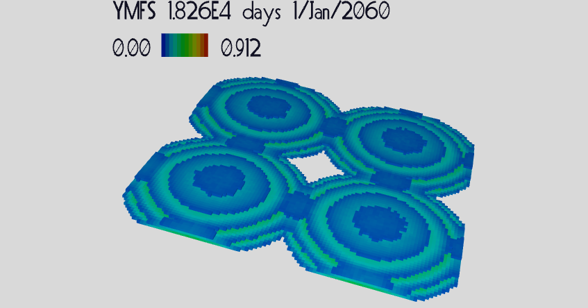
Advancing further in time, until the end of the simulation (2060), the CO2 is flattening-out due to the effect of diffusion in the vapour phase.
Analyse the results with ResInsight
Launch ResInsight, and load the “DEP_GAS.GRID” file. Then plot the field average pressure:
During depletion the pressure drops from 300 Bar to about 130 Bar, then it recovers to 150 Bars with the injection of CO2, and remains stable until the end of the simulation.
For the dynamic variable select YMFS, then select “Property Filters”:
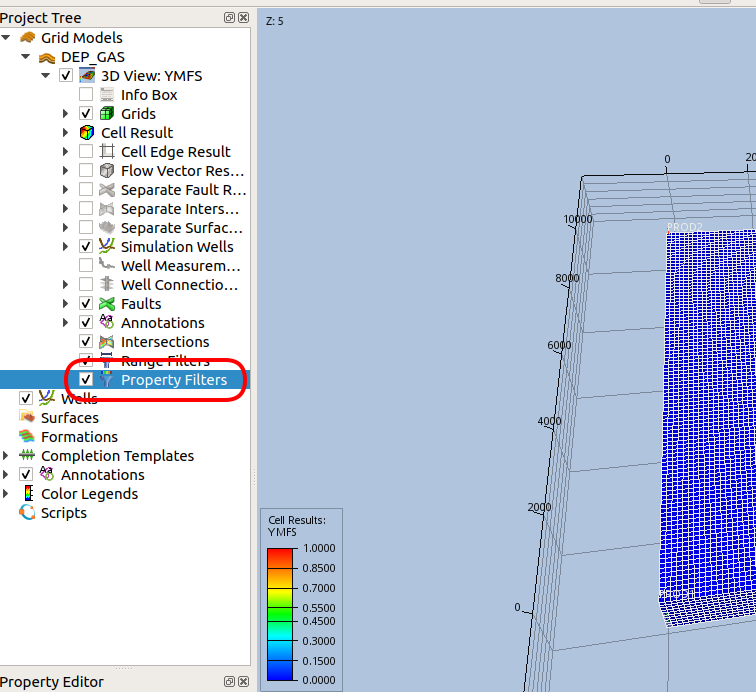
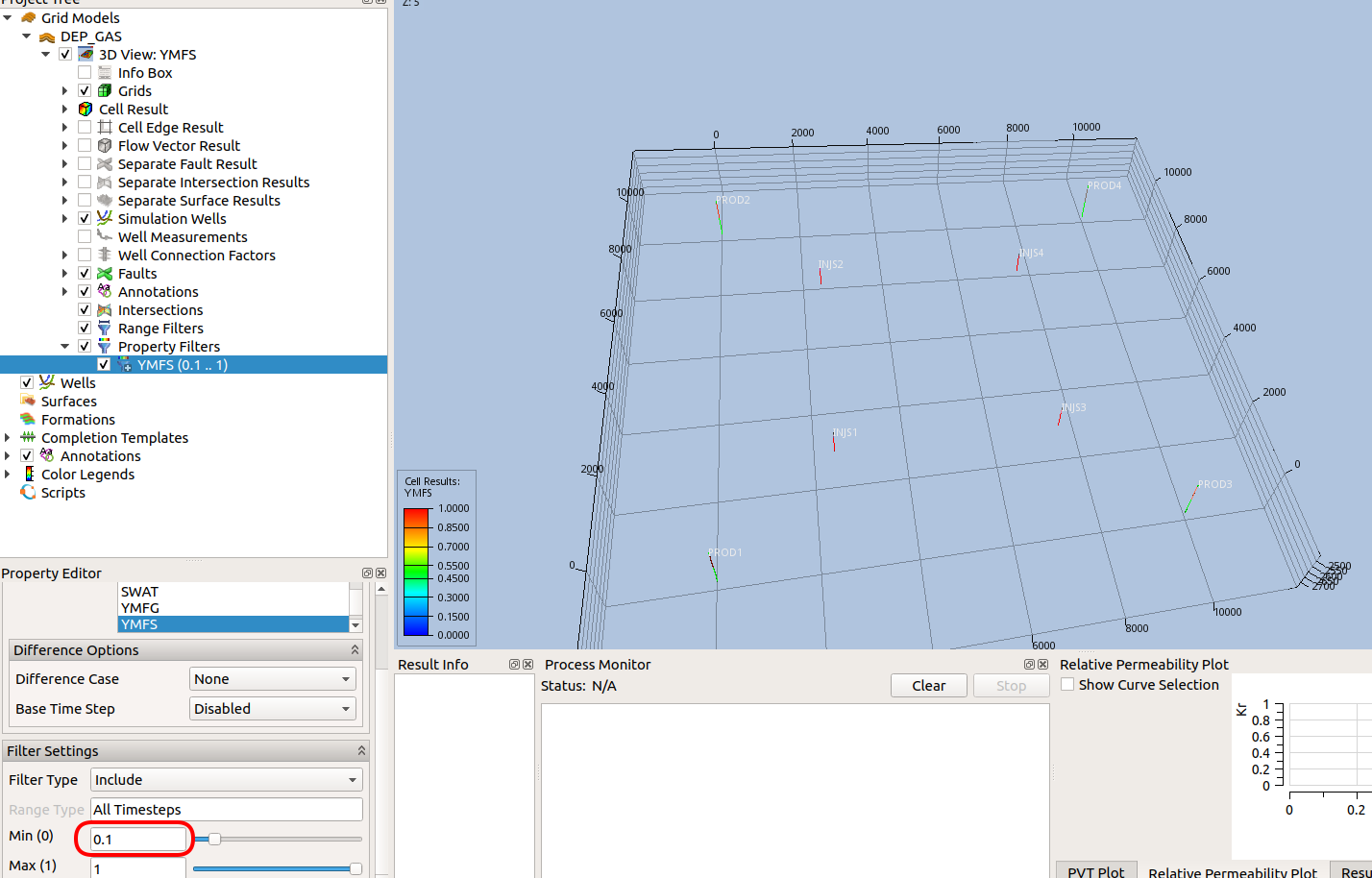
Then right-click and select “New Property Filter”. In the bottom left corner, under the Property Editor select 0.1 as minimum display threshold for the the 3D contour of YMFS, and type enter:
Advance the time until the end of the injection (1 Jan 2040):
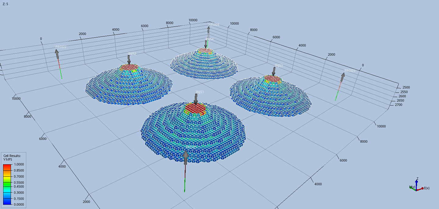
The plot above shows how the CO2, being heavier than the reservoir gas moves towards the bottom of the layer, above the gas-water contact.
Advancing further in time until the end of the simulation (2060), the CO2 is flattening-out due to the effect of diffusion in the vapour phase.